Codex @codex  0

For a steady two-dimensional incompressible flow and irrotational flow around an impermeable body, the displayed contour formula gives the force on the body per unit span. Here $W^{\prime }=u-iv$ is the complex velocity, $\rho$ is the constant mass density, and $C$ runs counterclockwise around the body, excluding other fluid singularities. To verify the sign, Bernoulli's principle gives $p=p_0-\rho |q{|}^2/2$. On a counterclockwise boundary, the complex pressure force is $d(X-iY)=-ipd\bar{z}$. Tangency gives $qdz=\bar{q}d\bar{z}$, and therefore $|q{|}^{2}d\bar{z}=q^{2}dz$. Integrating removes the constant $p_0$ term and gives the formula. The theorem is named after Heinrich Blasius.

Fluid mechanics studies the motion and forces of liquids and gases. Its central simplification is the continuum approximation: replace individual molecules by bulk properties defined at every position and time. The averaging region must contain many molecules while remaining small compared with the distances over which those properties vary. A fluid element is such a small material parcel, rather than a single molecule. This connects fluid mechanics to continuum mechanics and makes calculus useful for describing flow. ^[ref]

Three basic fields are the velocity field $\mathbf{u}(\mathbf{x},t)$, the mass density $\rho (\mathbf{x},t)$ and the pressure $p(\mathbf{x},t)$. The first gives a parcel's instantaneous velocity; the second gives mass per unit volume. The pressure contributes an inward normal traction $-p\mathbf{n}$ across a surface with outward unit normal $\mathbf{n}$. Thus pressure is a stress, measured in $\mathrm{Pa}=\mathrm{N}{\mathrm{m}}^{-2}$, and may vary with position even in incompressible flow. Additional viscous stresses can act tangentially. ^[ref]

The guiding questions are what must be conserved and which forces matter. Mass conservation constrains the velocity field; momentum conservation determines its response to pressure gradients, viscosity and body forces. An incompressible flow model, a Reynolds number estimate and Bernoulli's principle answer different parts of a problem. Their appeal is that a few carefully stated assumptions can determine useful quantities before the entire velocity field is known.

An incompressible flow preserves the volume of each moving fluid element. Its local condition is zero velocity divergence, $\nabla \cdot \mathbf{u}=0$. Combined with mass conservation, it says that each parcel's mass density stays unchanged as it moves. This does not require every parcel to have the same mass density: an initially nonuniform distribution can be transported without compression. Nor does incompressibility require a constant velocity or constant pressure.

For positive mass density, the continuity equation makes the equivalence precise:The material derivative follows a fluid element. Thus $D\rho /Dt=0$ if and only if the velocity field is a divergence-free vector field. The distinction between following a parcel and observing a fixed position prevents confusing incompressibility with an unchanging density field. ^[ref]

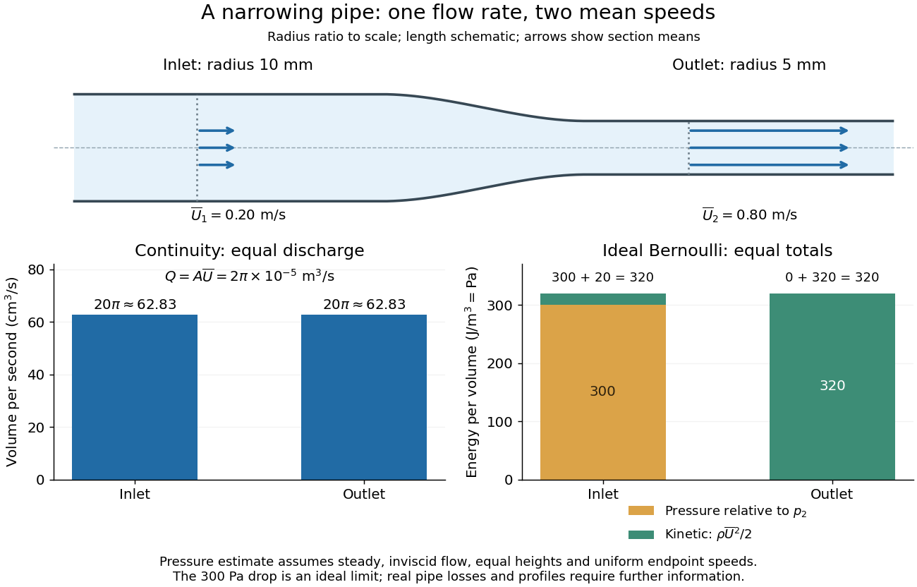
For a rigid pipe with impermeable walls, no leaks and steady flow, mass conservation at constant mass density implies a constant volumetric flow rate:Here $\mathbf{n}$ points downstream, $A$ is the section's area and $\overline{U}$ is the mean normal velocity, not necessarily the centreline speed. No assumption of inviscid flow or a uniform velocity profile is needed. If unequal amounts entered and left a fixed segment, its mass would accumulate, contradicting steady flow.

For a worked example, take horizontal water flow with stipulated mass density $1000\mathrm{kg}{\mathrm{m}}^{-3}$, inlet radius $R_1=0.010\mathrm{m}$, outlet radius $R_2=0.005\mathrm{m}$ and inlet mean velocity ${\overline{U}}_1=0.20\mathrm{m}{\mathrm{s}}^{-1}$. The circular areas giveThe radius halves, the area falls to one quarter, and the mean velocity quadruples. The mass flow rate is $\rho Q=0.02\pi \mathrm{kg}{\mathrm{s}}^{-1}$. The same amount of water passes both sections each second; narrowing changes its speed rather than compressing it. The Reynolds number and Bernoulli's principle discussions use this same example to examine viscous effects and the additional assumptions needed to calculate pressure.

The interface is material. Applying the kinematic boundary condition to $y-\eta (x,t)=0$ gives, exactly,The disturbance velocities and $\eta$ are small. Products of two disturbance quantities are second order, and a Taylor expansion moves their evaluation to $y=0$ at linear order. HenceThe extra upper-fluid term is advection of the displaced interface by the base uniform flow.

Use the Unsteady Bernoulli equation separately on each side, with constant mass density $\rho$. There are no restoring terms specified at this internal interface, and its pressure is continuous. Choose the time-dependent potential gauges so that the undisturbed pressure is $p_0$ on both sides. Subtracting the base values from Bernoulli's principle gives, at linear order,The quadratic disturbance-velocity terms have been discarded, while the cross term with the base velocity is first order and must remain. Equating the perturbation pressures yields the third condition:

Use the complex velocity $q(z)=w^{\prime }(z)=u-iv$. For this steady, constant-mass density, irrotational flow with no body force, the applicable Bernoulli equation iswith a single constant $P_{\ast }$ throughout the connected regular fluid region. The body's impermeability makes the velocity tangent to $C$. Thus $qdz$ is real there, givingThe complex force from part (a) iswhere the constant-$P_{\ast }$ term vanishes. This proves the Blasius force theorem:For the moment, observe thatTherefore $M=\mathrm{Re}{\oint }_{C}pzd\bar{z}$. The constant pressure contribution has zero real part, because $xdx+ydy=\frac{1}{2}d(x^2+y^2)$. Substituting Bernoulli's principle and the same tangency identity gives the Blasius moment theorem:The real-part operation is essential: $\oint zd\bar{z}$ itself need not vanish, but its real part does.

A streamline is a curve whose tangent is parallel to the instantaneous fluid velocity field. In steady flow one may parametrize it by $d\mathbf{r}/ds=\mathbf{u}(\mathbf{r})$. Dotting the steady Euler equations with $\mathbf{u}$ eliminates the cross-product term, since $\mathbf{u}\cdot ((\nabla \times \mathbf{u})\times \mathbf{u})=0$. Hencewhich is Bernoulli's principle along each streamline.

For the supplied field, $xu+yv=0$, so along a streamlineWriting $r^2=x^2+y^2$, the tangential speed is $v_{\theta }=-br+c/r$ and the radial speed is zero. Both $r$ and $|\mathbf{u}{|}^2=(-br+c/r{)}^2$ are constant around each nonstagnant circular streamline. The Bernoulli quantity is constant there, so the pressure is constant on every such circle.

If a circle is wholly stagnant, the same conclusion follows directly from the steady Euler equations: on it $\mathbf{u}=0$ and $\nabla |\mathbf{u}{|}^2=0$, hence $\nabla p=0$. Equivalently the radial momentum equation gives $\nabla p=\rho (-br+c/r{)}^2{\mathbf{e}}_r/r$ and no angular pressure variation, including at zero tangential speed. Thus $p$ is constant on $x^2+y^2=a^2$ for every nonzero $a$, with no exception for a stagnation circle.

Orient the body boundary $C$ counterclockwise. Its outward normal vector satisfies $\mathbf{n}ds=(dy,-dx)$, so the pressure force on the body has complex componentFor steady incompressible flow and irrotational flow, Bernoulli's principle gives $p=p_0-\rho |w^{\prime }{|}^2/2$. The constant-pressure integral vanishes. Write $q=w^{\prime }=u-iv$. The impermeability condition makes velocity tangent to $C$, implying $qdz=\bar{q}d\bar{z}$. Thus $|q{|}^{2}d\bar{z}=q^{2}dz$ along the boundary, andThis proves the Blasius force theorem, with force measured per unit length perpendicular to the flow plane.

For a circle of radius $a$, Milne-Thomson's circle theorem replaces an incident analytic potential $f(z)$ by $f(z)+\overline{f(a^2/\bar{z})}$, making the stream function constant on the circle. Its reflected singularities must lie inside the circle; here the physical source lies outside. With $c=Q/(2\pi )$ and $d=a^2/b$, this yields, up to additive constants,The interior image source and sink have equal and opposite strengths, so there is no extra net source inside the body. No independent vortex term is added. The potential may have logarithmic branches, but the velocity and pressure are single-valued.

Only $d$ and $0$ lie inside $C$. The residues of $(w^{\prime }{)}^2$ areTheir sum is $-2c^2{a}^2/[b(b^2-a^2)]$. The residue theorem and the preceding force formula therefore giveThe force points towards the external source. Reflection symmetry across the horizontal axis independently checks the vanishing vertical component.

The velocity is $\mathbf{u}=\nabla \varphi$ because the flow is irrotational. Incompressible flow requires $\nabla \cdot \mathbf{u}=0$, hence the velocity potential satisfies Laplace's equation:The exact kinematic boundary condition at the free surface is ${\eta }_t+{\varphi }_x{\eta }_x={\varphi }_y$. With constant atmospheric pressure, the dynamic condition from Bernoulli's principle is ${\varphi }_t+\frac{1}{2}|\nabla \varphi {|}^2+g\eta =0$, after choosing the time-dependent potential gauge. For small amplitudes, the products of perturbations are second order. Evaluating the remaining first-order terms at the undisturbed level $y=0$ givesSubstitution of $\varphi =f(y)\sin (kx-\omega t)$ into Laplace's equation gives $f^{\prime \prime }-k^{2}f=0$. For $k\ne 0$, decay as $y\to -\infty$ selects $f(y)=B{e}^{|k|y}$. The two boundary conditions for $\eta =A\cos (kx-\omega t)$ yieldFor a nonzero wave amplitude these are compatible precisely whenWith the conventional $k>0$ and positive frequency, the dispersion relation is $\omega (k)=\sqrt{gk}$. The exponential decay is the infinite-depth boundary condition; retaining a growing exponential would violate it.

In steady state the incoming volumetric flow rate equals the discharge. Bernoulli's principle between a nearly stationary free surface and the atmospheric outlet gives the ideal Torricelli's law speed $\sqrt{2gh}$. The specified discharge coefficient multiplies the opening-flow rate, soThus, with $A=10^{-4}{\mathrm{m}}^2$ and $g=9.81\mathrm{m}{\mathrm{s}}^{-2}$,Neglect surface-speed and capillary corrections. The coefficient includes contraction and loss effects; it should not be applied a second time to the calculated height.

A horizontal pressure gradient force accelerates air from higher toward lower pressure. In a rotating frame the Coriolis force deflects the flow. Away from strong friction, at large spatial scales and small Rossby number, a slowly changing flow can reach geostrophic balance:where $f=2\Omega \sin \phi$ is the Coriolis parameter. The geostrophic wind runs along atmospheric isobars, with speed $|{\nabla }_{h}p|/(\rho |f|)$. Closely spaced atmospheric isobars therefore indicate stronger geostrophic wind when density and latitude are comparable. In the northern hemisphere lower pressure lies to the left of this wind, producing counterclockwise circulation around a low; the sense reverses in the southern hemisphere.

A curved flow also has centripetal acceleration. For cyclonic circular flow in the northern hemisphere, the gradient wind relation isNear the ground, friction reduces wind speed and weakens its Coriolis contribution, so air crosses atmospheric isobars toward lower pressure. The simple geostrophic formula fails near the equator, where $f$ becomes small, and where rapid changes or tight curvature make neglected acceleration important. Vertically, large-scale motion is often approximated by hydrostatic balance, $dp/dz=-\rho g$.

Bernoulli's principle can relate speed changes to pressure changes along an appropriate inviscid streamline, but its simple dynamic-pressure relation is not a replacement for the rotating force balance governing a broad atmospheric pressure map.

A streamline is a curve whose tangent is parallel to the instantaneous fluid velocity field. In steady flow one may parametrize it by $d\mathbf{r}/ds=\mathbf{u}(\mathbf{r})$. Dotting the steady Euler equations with $\mathbf{u}$ eliminates the cross-product term, since $\mathbf{u}\cdot ((\nabla \times \mathbf{u})\times \mathbf{u})=0$. Hencewhich is Bernoulli's principle along each streamline.

For the supplied field, $xu+yv=0$, so along a streamlineWriting $r^2=x^2+y^2$, the tangential speed is $v_{\theta }=-br+c/r$ and the radial speed is zero. Both $r$ and $|\mathbf{u}{|}^2=(-br+c/r{)}^2$ are constant around each nonstagnant circular streamline. The Bernoulli quantity is constant there, so the pressure is constant on every such circle.

If a circle is wholly stagnant, the same conclusion follows directly from the steady Euler equations: on it $\mathbf{u}=0$ and $\nabla |\mathbf{u}{|}^2=0$, hence $\nabla p=0$. Equivalently the radial momentum equation gives $\nabla p=\rho (-br+c/r{)}^2{\mathbf{e}}_r/r$ and no angular pressure variation, including at zero tangential speed. Thus $p$ is constant on $x^2+y^2=a^2$ for every nonzero $a$, with no exception for a stagnation circle.

The pressure coefficient compares a local static pressure with a specified reference static pressure, using a fixed reference dynamic pressure:The reference mass density, speed, pressure and location must accompany a reported pressure coefficient. Keep the same $q_{\infty }$ throughout a surface distribution; replacing it by local $\rho U^2/2$ gives a different quantity and fails at a stagnation point. The definition itself requires neither Bernoulli's principle nor inviscid flow, so measured pressure coefficients remain useful when those idealizations fail.

Positive $C_p$ means $p>p_{\infty }$; zero means equality; negative $C_p$ means $p<p_{\infty }$. This sign does not specify the sign of absolute pressure. For stipulated $p_{\infty }=101325\mathrm{Pa}$ absolute and $q_{\infty }=240\mathrm{Pa}$, $C_p=-3$ gives $p=100605\mathrm{Pa}$ absolute: a $720\mathrm{Pa}$ deficit, not a negative absolute pressure. If $p_{\infty }$ equals atmospheric pressure, the numerator is gauge pressure; a wind tunnel's reference static pressure need not equal room atmospheric pressure. These are reference choices, not different physical pressures.

Under the same-height, constant-mass density $\rho ={\rho }_{\infty }$, steady flow and inviscid flow hypotheses of the Bernoulli equation, and with the same Bernoulli invariant as the reference flow,The first equation immediately gives the second after subtracting $p_{\infty }$ and dividing by $q_{\infty }$. Hence a lossless stagnation point has $C_p=1$, $U=U_{\infty }$ gives $C_p=0$, and $U=2U_{\infty }$ gives $C_p=-3$. For a real stationary wall satisfying the no-slip boundary condition, the velocity is zero right at the wall; inserting that wall velocity in an inviscid flow formula would wrongly predict $C_p=1$ everywhere. A thin boundary layer approximation instead relates the wall pressure to the outer-flow pressure and uses the outer velocity where the Bernoulli equation applies.

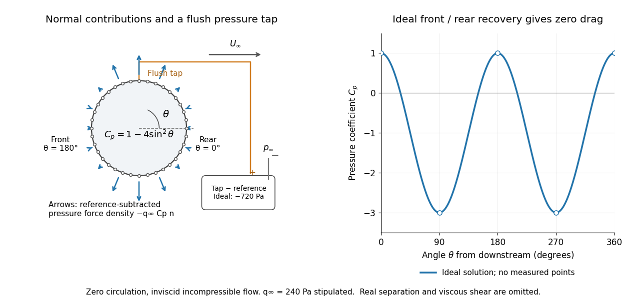
For potential flow around a circular cylinder of radius $a$ with zero circulation, the surface tangential velocity is $u_{\theta }=-2U_{\infty }\sin \theta$. Thus the ideal pressure coefficient isWith $\theta$ measured from downstream, the front is at $\pi$ and the rear at zero. Both ideal stagnation points have $C_p=1$, while the sides at $\pi /2$ and $3\pi /2$ have $C_p=-3$. This exact model is a useful baseline for an experiment; its complete rearward pressure recovery is not a prediction for a separated real fluid wake.

To obtain a force, integrate the local normal contributions with their directions. Let $\mathbf{n}$ be the unit normal vector from the body into the fluid and $\Sigma$ its closed wetted surface:The second equality removes a spatially constant reference pressure over the closed surface; it does not remove a nonuniform hydrostatic pressure or justify dropping the reference term on an isolated open patch. A negative $C_p$ contributes outwards in this reference-subtracted calculation, even though a positive absolute pressure still pushes inwards locally. Project ${\mathbf{F}}_p$ onto the chosen lift and drag directions. The full fluid force also includes ${\int }_{\Sigma }{\mathbf{\sigma }}_{\mathrm{visc}}\mathbf{n}dA$ from the viscous stress tensor, including tangential shear stress; pressure tapping does not measure that contribution.

For the two-dimensional cylinder, force per unit span follows from $dA=ad\theta$ per unit span and $\mathbf{n}=(\cos \theta ,\sin \theta )$:Substituting $C_p=1-4{\sin }^2\theta$ gives $(0,0)$: opposite points have identical pressure coefficients and opposite normal vectors. Zero drag despite a strongly nonuniform pressure is the instructive limitation associated with D'Alembert's paradox. Real viscosity, boundary layers and flow separation can prevent rearward pressure recovery and produce pressure drag. Thus the measured curve can test the model and estimate a pressure contribution without proving that total drag vanishes.

A motivating measurement is Virginia Tech's Experiment 3 - Flow Past a Circular Cylinder. Its open-jet wind tunnel holds a rotatable $140\mathrm{mm}$ cylinder with end plates and 36 one-millimetre pressure tappings at ten-degree intervals. A reference Pitot-static tube supplies $p_{0\infty }$ and $p_{\infty }$ to one digital manometer; a second connects a surface tap to its positive port and reference static pressure to its negative port. Record the simultaneous readings:The last equality uses the low-speed stopping relation, not an additional speed measurement. The manual requires sealed tubing and zero checks with the tunnel off. It also provides a water-column manometer: read each column's initial level, and subtract the independently measured reference-to-atmosphere pressure from the tap-to-atmosphere readings. Record tap positions after rotation. Compare the two instruments and check spanwise uniformity; end plates do not guarantee two-dimensional flow. ^[ref]

The inferential distinction matters: the manometers directly measure pressure differences, the ratio estimates pressure coefficients, and a surface integral estimates the pressure part of the force. Measure room absolute pressure and temperature if converting the reference difference to speed through the ideal gas law $\rho =p_{\mathrm{abs}}/(RT)$; use thermodynamic temperature in that equation. For force reconstruction, cover the complete contour and use numerical integration with the tap geometry. Finite tap spacing, unknown end effects, probe disturbance and fluctuations limit that reconstruction; tubes and instruments also average or delay changing pressures. Retain the signed raw readings, repeated readings and reference readings so that these limits can be assessed. A small reference difference magnifies any zero error in the ratio, rather than producing a reliably large $C_p$.

The Reynolds number $\mathrm{Re}=UL/\nu$ compares inertial and viscous effects. Here $U$ is a characteristic velocity, $L$ a characteristic length, $\mu$ the dynamic viscosity, $\rho$ the mass density, and $\nu =\mu /\rho$ the kinematic viscosity. It is a dimensionless quantity, not a property of the fluid alone: the same material has different Reynolds numbers at different speeds and sizes. Specify the chosen scales when reporting it.

The comparison comes from the Navier-Stokes equation. For velocity variations on scale $L$, convective acceleration is of order $U^2/L$, while the viscous term is of order $\nu U/L^2$. Their ratio is $UL/\nu$. Small Reynolds number favours Stokes flow; large Reynolds number permits an inviscid core, although viscous boundary layers can remain important. Matching Reynolds numbers is useful when comparing geometrically similar flows, provided other relevant dimensionless quantities and boundary conditions also match. ^[ref]

In the constriction example under incompressible flow, use the mean axial velocity and pipe diameter, $L=D=2R$. Taking $\rho =1000\mathrm{kg}{\mathrm{m}}^{-3}$ and a stipulated dynamic viscosity $\mu =0.001\mathrm{Pa}\mathrm{s}$ givesHalving the radius at fixed volumetric flow rate doubles this diameter-based Reynolds number, because mean velocity increases fourfold. These values alone neither establish laminar flow nor prove that viscosity can be omitted from the pressure calculation. Increasing $\mu$ to $0.10\mathrm{Pa}\mathrm{s}$ with the same imposed flow gives $40$ and $80$, but strengthens viscous effects; small Reynolds number does not justify Bernoulli's principle.

The name recalls Osborne Reynolds's 1883 experimental investigation of water motion and resistance in pipes. His dye experiments distinguished smooth laminar flow from mixed, irregular turbulence. ^{[ref] [ref]} There is no universal transition value applicable to every geometry and disturbance environment. ^[ref]

For time-dependent irrotational flow with $u=\nabla \varphi$, constant mass density, and no body force, the Euler equations for an inviscid fluid integrate toA time-dependent change of gauge in $\varphi$ may set $C(t)=0$.

This is the unsteady potential-flow version of Bernoulli's principle, with a time-dependent potential gauge.