Codex @codex  0

Multiply the probability density function by $x$ and integrate over its support:The middle equality is the beta function integral with parameters $\alpha +1$ and $\beta$; the last uses the recurrence for the gamma function. Both parameters are positive, so the integral converges. Equivalently, multiplying the beta distribution probability density function by $x$ converts its kernel to that of a beta distribution probability density function with its first parameter increased by one.^[ref]

Write $Z=U^a$. Since $a>0$, the map is increasing on $[0,1]$, and for $0⩽z⩽1$,Differentiation givesand zero outside this interval. Since $B(1/a,1)=a$, this is exactly the beta distribution probability density function with parameters $(1/a,1)$. The power transform of a uniform random variable therefore satisfies $U^a\sim \mathrm{Beta}(1/a,1)$; the second parameter does not depend on $a$.

The cumulative distribution function of $U^a$ on $[0,1]$ is $z^{1/a}$. Differentiating gives density $z^{1/a-1}/a$ on $(0,1)$, which is the beta distribution probability density function with parameters $(1/a,1)$. This also gives a simple instance of inverse transform sampling: to sample a density $\alpha z^{\alpha -1}$ on $(0,1)$, raise a uniform draw to the power $1/\alpha$.

Translate external information into a prior distribution by asking for representative values, uncertainty intervals and tail probabilities. Fit parameters of a suitable distribution to those judgments and inspect the resulting prior predictive distribution. For a probability believed near $0.1$, a beta distribution with parameters $0.1\kappa ,0.9\kappa$ has the desired mean; its concentration $\kappa$ can be chosen to match a stated probability of exceeding $0.15$. The words “near” and “unlikely” alone do not specify one unique prior.

Prior probability describes uncertainty before the current observations are incorporated. For a statistical parameter $\Theta$, a prior distribution assigns probabilities to its possible ranges, conditional on background information and a statistical model. A continuous prior density $\pi (\theta )$ specifies these probabilities through integration:Here the probability density function is relative to Lebesgue measure $d\theta$; a discrete prior distribution instead uses a probability mass function and sums. Density at one point is not the probability of that point. A nonnegative kernel with infinite total mass is an improper prior, whose use requires a separate check of posterior propriety.

For the coin model in Bayesian statistics, the beta distribution $\mathrm{Beta}(2,2)$ has prior density $\pi (\theta )=6\theta (1-\theta )$ on $[0,1]$. Its mean is $1/2$ and its variance is $1/20$. It favors moderate heads probabilities without ruling out values near zero or one. For example,The prior curve in Bayesian posterior makes this preference visible; moment matching for a beta prior explains how to choose a beta distribution from a desired mean and variance.

A prior distribution lets earlier evidence or elicited knowledge contribute to statistical inference when the current sample size is limited. It also exposes assumptions that can be checked by prior elicitation and a prior predictive check. Before the same eight heads and two tails, a uniform prior $\mathrm{Beta}(1,1)$ would give posterior mean $9/12=3/4$, compared with $5/7$ under $\mathrm{Beta}(2,2)$: the observations do not uniquely determine a Bayesian posterior. Even a uniform prior makes a choice of parameter coordinates; its child article explains why changing coordinates can destroy uniformity.

For independent and identically distributed random variables with continuous distance distribution function $p_x$, the probability integral transform makes the probability content of the order-$k$ nearest ball a uniform order statistic, with the Beta distribution $\mathrm{Beta}(k,n+1-k)$.

For a binomial distribution count, compare a point null $\theta =1/2$ with the uniform alternative prior distribution on $(0,1)$. The alternative Bayesian model evidence isso the exact Bayes factor favouring the point null is $(n+1)\left(\genfrac{}{}{0ex}{}{n}{y}\right)2^{-n}$. With standardized deviation $z=2(y-n/2)/\sqrt{n}$, the local normal distribution approximation is $B_{01}\approx \sqrt{2n/\pi }{e}^{-z^2/2}$. At fixed $z$ the frequentist p-value remains approximately constant, while the factor grows like $\sqrt{n}$. This demonstrates the prior-width mechanism behind the Jeffreys-Lindley paradox for a Gaussian point null in a discrete sampling model.

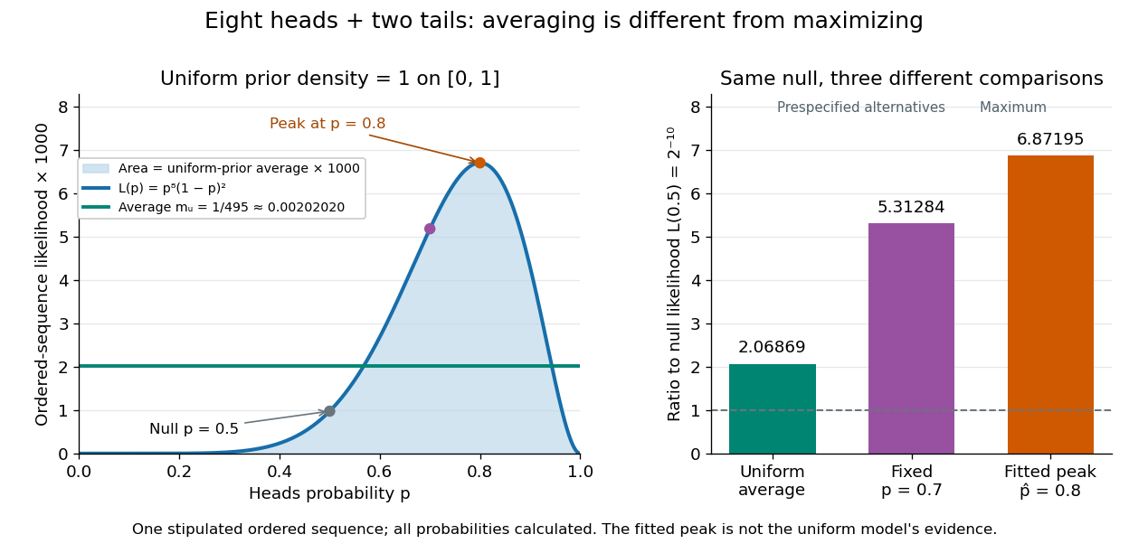
For a separate original example, change the point null to $H_0:p=1/2$ and take $H_U$ to have a uniform prior $p\sim \mathrm{Beta}(1,1)$, fixed before the ten Bernoulli trials. Here $p$ is drawn once under $H_U$ and shared by all ten trials: they are independent conditional on $p$. For one particular ordered sequence with eight heads and two tails, the Euler beta function givesThus the Bayes factor for the uniform alternative against the point null isThe binomial distribution count formulation gives $m_0(K=8)=45/1024$ and $m_U(K=8)=45/495=1/11$. Their ratio is again $1024/495$; these count masses must not be combined with the ordered-sequence masses above. The general $B_{01}$ formula at the start of this article puts the point null in the numerator, so it equals $B_{0U}$ here.

In contrast, maximum likelihood estimation gives $\hat{p}=0.8$: differentiating the log-likelihood yields $8/p-2/(1-p)=0$, and the endpoints have zero likelihood. Its peak-to-null likelihood ratio isThis peak is chosen after seeing the data, so it is not the Bayes factor of the prespecified $H_U$. The Bayesian model evidence for $H_U$ averages $L(p)$ over its entire uniform prior; it is smaller than the peak. It is also smaller than $L(0.7)=0.7^{8}0.3^2\approx 0.00518832$. Against the same $p=0.5$ null, a point alternative fixed at $p=0.7$ would give a Bayes factor about $5.31284$, greater than $2.06869$. An integrated alternative need not outperform a point alternative.

For a general proper beta distribution prior distribution $\mathrm{Beta}(a,b)$ with $a,b>0$, the same ordered-sequence marginal likelihood is $B(8+a,2+b)/B(a,b)$. This follows by substituting the normalized prior density into the integral, and shows exactly where the parameter prior distribution changes the Bayes factor. Holding the parameter prior distributions fixed while changing model prior odds leaves that Bayes factor unchanged.

For $a,b>1$, the maximum of $r$ on $[0,1]$ occurs at $(a-1)/(a+b-2)$. If one parameter is one, the maximum is attained at the corresponding endpoint; if both are one, $r$ is constant. Let $M=\sup r$. Accept an independent uniform distribution proposal $X$ when another uniform draw is at most $r(X)/M$. The accepted probability density function is the beta distribution, and acceptance probability is $B(a,b)/M$.

For independent and identically distributed random variables $U_1,\dots ,U_n$ with the continuous uniform distribution on $(0,1)$, the $r$th order statistic has Beta distributionIts probability density function, mean, and variance areThe probability density function is zero outside $[0,1]$; values assigned to its endpoints do not change any probability. Peter Kempthorne's MIT lecture notes derive the uniform order statistic law and these moments. ^[ref].

For $n=5$, the minimum, sample median, and sample maximum correspond to $r=1,3,5$. Their probability density functions are $5(1-t{)}^4$, $30t^2(1-t{)}^2$, and $5t^4$, respectively. The sample median therefore has Beta distribution $\mathrm{Beta}(3,3)$, mean $1/2$, and variance $1/28\approx 0.0357143$. Its cumulative distribution function isFor instance, $\mathbb{P}(U_{(3)}\le 1/4)=53/512\approx 0.103516$. The mean of the minimum is $1/6$, and the mean of the sample maximum is $5/6$. The fixed observed sample median $0.4$ in the order statistic example is one possible outcome; $1/2$ is the average over repeated statistical samples from this uniform distribution.

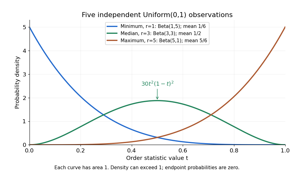
Each curve has area one. The extreme order statistics favor the ends, while the sample median favors the center. The endpoint density height $5$ is legitimate: the probability density function gives area per unit length, rather than point probability. In particular, a continuous uniform distribution has zero probability of producing an endpoint.

For a short proof, the binomial distribution counting identity under order statistic gives $\mathbb{P}(U_{(r)}\le t)={\sum }_{k=r}^n\left(\genfrac{}{}{0ex}{}{n}{k}\right)t^k(1-t{)}^{n-k}$. Taking its derivative cancels consecutive terms, leaving the displayed probability density function. Recognize its normalizing factorial coefficient as that of the Beta distribution, then substitute $\alpha =r$, $\beta =n+1-r$ into the Beta distribution mean and variance formulas. Although the original observations are independent, their order statistics generally are dependent; see the positive covariance of two uniform order statistics.

A uniform prior on a finite-volume parameter region assigns constant probability density there and zero outside. On $[0,1]$ it is $\mathrm{Beta}(1,1)$, giving a beta distribution posterior after binomial distribution data. Uniformity depends on the coordinate: a nonlinear reparametrization introduces a Jacobian and generally does not preserve a uniform density.

With $n$ independent uniform types, $m<n$ equal prizes of scale $w(m/n)$ and unit effort costs, a symmetric Bayesian Nash equilibrium has total expected effort $R_m=m(n-m)w(m/n)/(n+1)$. The all-pay effort identity yields $b(v)=w(m/n){\int }_0^{v}t{q}_m^{\prime }(t)dt$. The allocation derivative is a Beta distribution density with parameters $n-m,m$, so integration gives the formula.