Codex @codex  0

The standard arcsine distribution is a continuous probability distribution on $[0,1]$ with probability density functionIt is the beta distribution with both parameters equal to $1/2$. The density grows without bound toward both endpoints, yet neither endpoint has any probability mass. Its name comes from the inverse sine in its cumulative distribution function.^[ref]

A useful way to see the shape is to choose a point uniformly around a circle and project it onto a diameter. Equal angular intervals do not give equal horizontal distances: the projection moves slowly near either end. An ideal harmonic oscillator sampled at a uniformly chosen time in one complete period has the same endpoint concentration after rescaling its position. The distribution translates a simple geometric slowdown into a precise probability calculation.

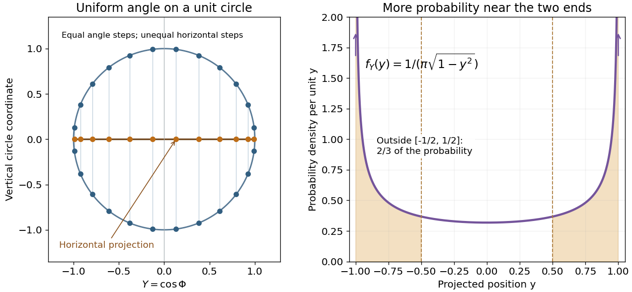
For an original comparison, take equal-length regions: the middle half $[1/4,3/4]$, and the two outside quarters together. ThenA uniform distribution on $[0,1]$ instead assigns each region probability $1/2$. Both distributions have mean $1/2$; the mean alone hides their different concentration.

Bayesian statistics expresses uncertainty about an unknown statistical parameter through a probability distribution, then uses Bayes' theorem to update it after observing data. The prior distribution describes uncertainty before the current observations; the likelihood function describes how the statistical model generates those observations at each parameter value; the posterior distribution describes uncertainty conditional on the observations and that model. A physical parameter can have one fixed value while its value remains uncertain to us. Assigning it a probability distribution represents that uncertainty under the chosen model, rather than requiring the physical parameter to change randomly between measurements.

For example, suppose ten Bernoulli trials are independent conditional on an unknown heads probability $\theta$, with a beta distribution prior $\mathrm{Beta}(2,2)$. Eight heads and two tails give the posterior distribution $\mathrm{Beta}(10,4)$ by Beta-binomial conjugacy. Its posterior mean is $10/14=5/7\approx 0.714286$, between the prior mean $1/2$ and observed binomial proportion $8/10$. The Bayesian posterior below computes the whole update, and the credible interval below summarizes its remaining uncertainty. The conjugate update is explained in MIT 18.05, Reading 15: beta and normal conjugate priors.

The useful feature is that one posterior distribution supports several questions: a posterior mean estimates a value, a credible interval reports a range, and a posterior predictive distribution predicts a future observation while averaging over parameter uncertainty. With conditionally independent new data, today's posterior distribution can become tomorrow's prior distribution. These conclusions remain conditional on the statistical model and prior distribution; a precise update does not establish that either assumption fits the experiment.

A historical starting point is Thomas Bayes's essay in the 1763 volume of the Royal Society's Philosophical Transactions, communicated after his death by Richard Price. Its opening problem asks for uncertainty about an unknown event probability given observed successes and failures: the same direction of reasoning illustrated by the coin example. See Bayes and Price, An Essay towards solving a Problem in the Doctrine of Chances, opening letter and problem.

Mix a binomial distribution with a beta distribution for its success probability: $\Theta \sim \mathrm{Beta}(\alpha ,\beta )$ and $Y\mid \Theta \sim \mathrm{Binomial}(n,\Theta )$. Integrating their densities gives the displayed mass for $y=0,\dots ,n$. Its expectation is $n\alpha /(\alpha +\beta )$, and its variance is $n\alpha \beta (\alpha +\beta +n)/[(\alpha +\beta {)}^2(\alpha +\beta +1)]$. It is the posterior predictive distribution for repeated Bernoulli trials after a beta-prior update.

Draw $P\sim \mathrm{Beta}(\alpha ,\beta )$, $X\mid P\sim \mathrm{Binomial}(n,P)$ and $Q\mid X\sim \mathrm{Beta}(\alpha +X,\beta +n-X)$, with $\alpha ,\beta >0$ and integer $n\ge 0$. The joint density of $(P,X,Q)$ is symmetric in $P,Q$, making them exchangeable random variables with identical beta distribution marginal distributions. The posterior beta normalization constant depends on $X$ and must be retained. The correlation coefficient is $n/(n+\alpha +\beta )$: this constructs tunable dependence without altering either marginal.

The beta distribution is an absolutely continuous probability distribution for a random variable $X$ between zero and one. It can describe uncertainty about a probability, such as an unknown coin's chance of heads. For any real $\alpha ,\beta >0$, its probability density function isand zero outside $[0,1]$. The normalizer is the Euler beta function, related to the gamma function by the beta-gamma identity:Thus the probability density function integrates to one. ^[ref].

The endpoint behavior explains why the restrictions are exactly $\alpha ,\beta >0$: near zero the probability density function behaves like a constant times $x^{\alpha -1}$, and near one like a constant times $(1-x{)}^{\beta -1}$. These improper integrals converge for positive parameters, even when the probability density function diverges at zero for $\alpha <1$ or at one for $\beta <1$. There is no probability mass at either endpoint: $\mathbb{P}(X=0)=\mathbb{P}(X=1)=0$. A probability density function's height is not a probability; an interval's probability is the area under it.

Some useful examples of the beta distribution are:

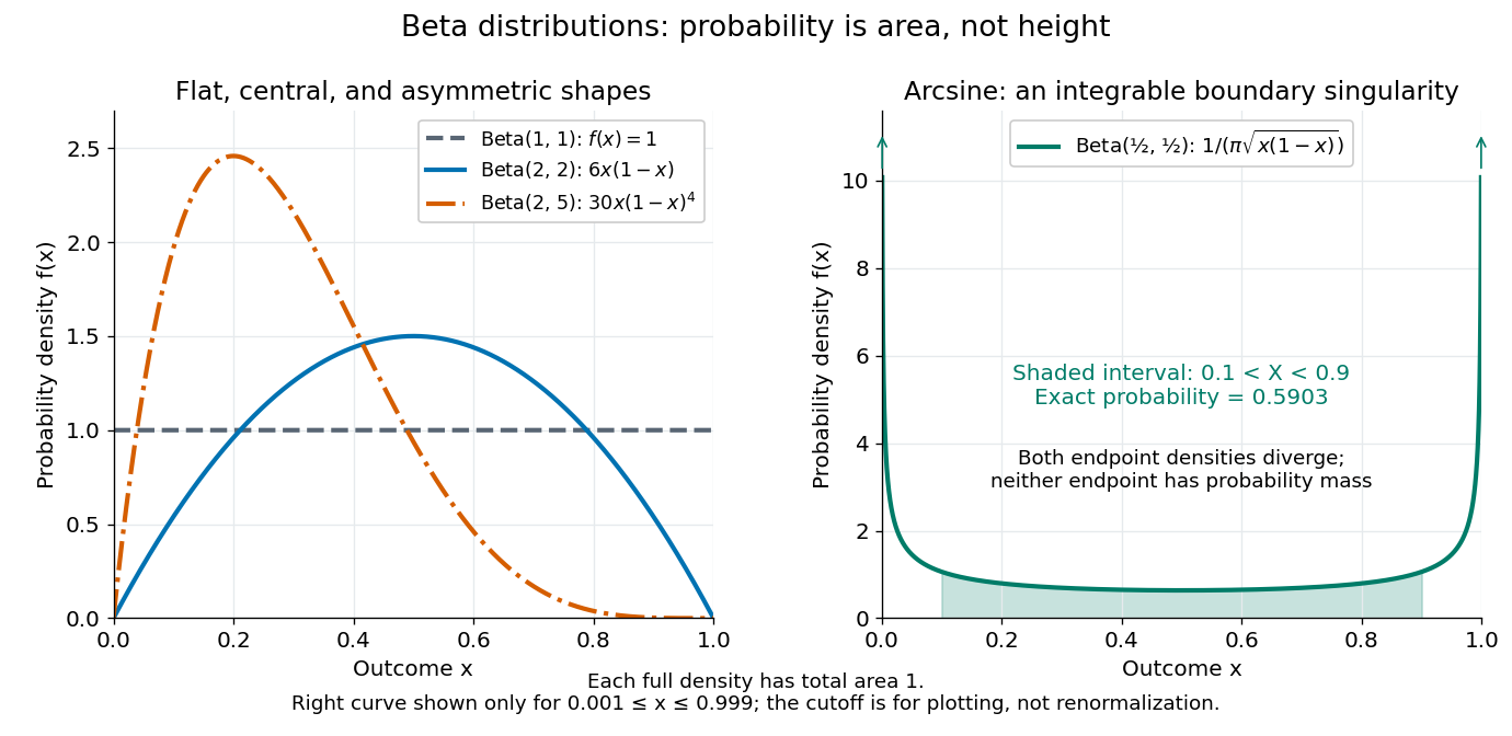
The arcsine distribution curve is plotted only for $0.001\le x\le 0.999$; its finite plotted ends do not represent finite endpoint values of the probability density function. Using the inverse sine, the shaded central interval has exact probability $\mathbb{P}(0.1<X<0.9)=1-4\arcsin (\sqrt{0.1})/\pi \approx 0.5903$, calculated analytically rather than by treating the cropped curve as normalized.

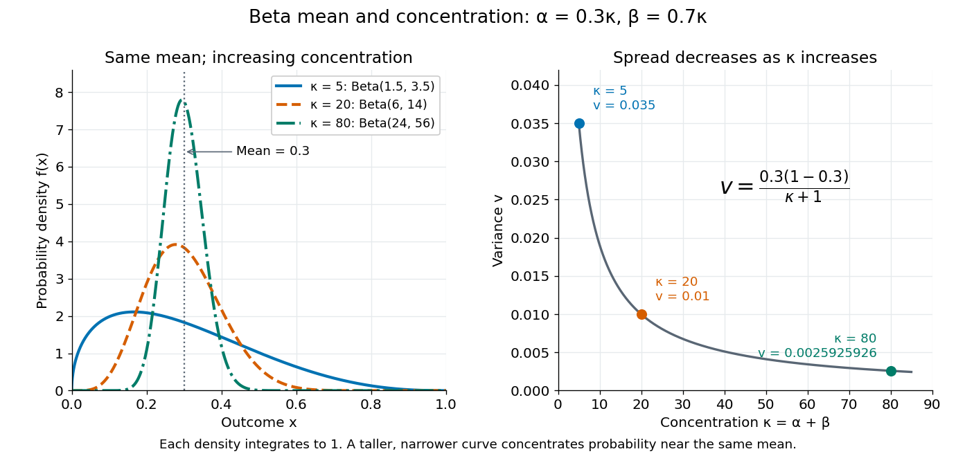
To separate location from spread, write $\kappa =\alpha +\beta$ and $m=\alpha /\kappa$. The mean and variance of the beta distribution areThe mean specifies the balance between the parameters; their sum $\kappa$ controls concentration about that mean. Multiplying both parameters by the same positive number preserves the mean and changes the variance. Larger $\kappa$ puts more area near $m$ and makes the probability density function taller there; the total area stays one. Small $\kappa$ allows much greater spread, sometimes favoring the endpoints rather than the mean itself.

For example, keeping mean $m=0.3$ and taking $\kappa =5,20,80$ gives the beta distributions $\mathrm{Beta}(1.5,3.5)$, $\mathrm{Beta}(6,14)$, and $\mathrm{Beta}(24,56)$. Their variances are $0.035$, $0.01$, and $0.21/81\approx 0.00259259$, respectively. Parameters need not be integers.

The formulas follow from two short moment calculations. Multiplying the probability density function by $x$ or $x^2$ increases the first parameter of the Euler beta function:Apply the Gamma function recurrence to the beta-gamma identity, then subtract $(\mathbb{E}[X]{)}^2$ from $\mathbb{E}[X^2]$ to obtain the variance.

The beta distribution is especially convenient as a prior distribution for the unknown success probability $P$ of Bernoulli trials. The Beta-binomial conjugacy says that $h$ successes and $t$ failures update a prior distribution $\mathrm{Beta}(\alpha ,\beta )$ to a posterior distribution $\mathrm{Beta}(\alpha +h,\beta +t)$. For example, suppose a coin has prior distribution $\mathrm{Beta}(2,2)$ and we observe eight heads and two tails. Its posterior distribution is then $\mathrm{Beta}(10,4)$, with posterior mean $5/7$. ^[ref].

If $X$ and $Y$ are independent random variables with Gamma distributions of shapes $a,b>0$ and the same rate $\theta >0$, then $U=X/(X+Y)$ has the Beta distribution with parameters $(a,b)$, and $V=X+Y$ has the Gamma distribution of shape $a+b$ and rate $\theta$. Moreover $U$ and $V$ are independent. The inverse change of variables $(x,y)=(uv,(1-u)v)$ has absolute Jacobian determinant $v$, which makes the joint probability density factorize on the product domain $0<u<1$, $v>0$. The common rate is essential for this factorization.

For independent geometric random variables with success probability $p$, observing $d$ terminal events and $F$ preceding failed Bernoulli trials gives likelihood function proportional to $p^d(1-p{)}^F$. Multiplication by a beta distribution prior $\mathrm{Beta}(a,b)$ gives the posterior distribution $\mathrm{Beta}(a+d,b+F)$. With complete waiting times $x_1,\dots ,x_n$, take $d=n$ and $F={\sum }_i(x_i-1)$.

A waiting time that is right-censored after $c$ failed trials contributes $(1-p{)}^c$: increase $F$ by $c$ without increasing $d$. This requires the censoring mechanism to be ignorable, as with an externally fixed observation horizon. Counting a censored waiting time as an observed event changes the likelihood function and biases the update.

For a beta distribution with shape parameters $A,B>1$, the probability density function vanishes at zero and one and is strictly increasing up to $m=(A-1)/(A+B-2)$ and strictly decreasing afterwards. This follows because the derivative of its logarithm is $(A-1)/t-(B-1)/(1-t)$, whose sign changes at $m$.

For each $0<\alpha <1$, the highest posterior density interval when this beta distribution is a posterior distribution has unique endpoints $0<l<m<u<1$ determined byThe second equation gives equal endpoint posterior densities. For every density threshold strictly between zero and the modal height there is precisely one crossing on each side. The enclosed probability is continuous and strictly decreasing from one to zero as the threshold increases, proving existence, uniqueness and the highest posterior density interval property. The restrictions $A,B>1$ are essential to this two-interior-endpoint characterization; monotone cases use a support boundary instead.

For $a,b>0$, this probability density function is obtained from a beta distribution variable $U$ by $X=U/(1-U)$. Indeed $u=x/(1+x)$ and $du/dx=(1+x{)}^{-2}$, and the change of variables formula gives the displayed density. In particular, the ratio of two independent equal-rate exponential distributions has $a=b=1$, density $(1+x{)}^{-2}$ and cumulative distribution function $x/(1+x)$.

Independent gamma distributions $S\sim \Gamma (\alpha ,r)$ and $T\sim \Gamma (\beta ,r)$ with a common rate yield a Beta distribution $S/(S+T)\sim \mathrm{Beta}(\alpha ,\beta )$. The change of variables $S=wu$, $T=w(1-u)$ has Jacobian determinant $w$, and factors the joint probability density function into a Beta distribution density in $u$ and a gamma distribution density in $w$. In particular, independent chi-squared distributions with $2\alpha$ and $2\beta$ degrees of freedom give the required ratio.

For positive integers $\alpha ,\beta$, the $\alpha$th order statistic from $\alpha +\beta -1$ independent uniform distributions on $(0,1)$ has Beta distribution $\mathrm{Beta}(\alpha ,\beta )$. Selecting the observations below and above a value $u$ gives its probability density function proportional to $u^{\alpha -1}(1-u{)}^{\beta -1}$, with normalizing factor $(\alpha +\beta -1)!/((\alpha -1)!(\beta -1)!)$.

For $m$ independent binomial distribution observations with fixed trial count $n$ and total successes $s$, the likelihood-power probability density function relative to $dp$ is $p^{s/T}(1-p{)}^{(mn-s)/T}$. Its normalized law is the displayed beta distribution. Its mean tends to $s/(mn)$ and its variance tends to zero as $T\downarrow 0$, including endpoint maxima. Energy for maximizing a log-likelihood is its negative; the opposite sign reverses the optimization.

In a normal linear model with residual degrees of freedom $\nu \ge 2$, an internally studentized residual satisfies $|{\eta }_i|\le \sqrt{\nu }$ and ${\eta }_i^2/\nu \sim \mathrm{Beta}(1/2,(\nu -1)/2)$, provided its leverage is less than one. Choose an orthonormal basis of the residual space with its first direction proportional to the projection of the $i$th coordinate vector. The Gaussian coordinates in this basis are independent standard normal random variables $Z_1,\dots ,Z_{\nu }$, and ${\eta }_i=\sqrt{\nu }{Z}_1/({\sum }_j{Z}_j^2{)}^{1/2}$. The beta distribution follows from the independent chi-squared distributions of $Z_1^2$ and ${\sum }_{j=2}^{\nu }{Z}_j^2$. The bounded residual is not exactly distributed according to Student's t-distribution; it approaches the standard normal distribution as $\nu \to \infty$.

An equal-tailed credible interval uses quantiles of a continuous posterior distribution to leave posterior probability $\alpha /2$ in each tail. It is also called a central credible interval; central refers to equal tail probabilities, not equal distances from the posterior mean. For the beta distribution $\mathrm{Beta}(10,4)$ in credible interval, the 95% endpoints are approximately $0.461868461$ and $0.909079605$, whose midpoint $0.685474033$ differs from the posterior mean $5/7$.

For an independent statistical sample from the beta distribution with parameters $(\theta ,1)$, $\theta >0$, the probability density function is $\theta x^{\theta -1}$ on $(0,1)$. Its raw moments are $\mathbb{E}{X}^r=\theta /(\theta +r)$ for $r>-\theta$, by direct integration. Consequently the method of moments gives $T_1=\bar{X}/(1-\bar{X})$, whereas the maximum-likelihood estimator is $T_2=-n/{\sum }_i\log X_i$.

The second formula follows by setting the score function $n/\theta +{\sum }_i\log X_i$ to zero; its derivative is negative. Also $-\log X_i$ has an exponential distribution of rate $\theta$, since $\mathbb{P}(-\log X_i>u)=e^{-\theta u}$. The central limit theorem and delta method giveThus the asymptotic relative efficiency of $T_1$ relative to $T_2$ is $1-(\theta +1{)}^{-2}$. The transformed sum has a gamma distribution of shape $n$ and rate $\theta$, which also gives $\mathbb{E}{T}_2=n\theta /(n-1)$ for $n>1$ and $\mathrm{Var}(T_2)=n^2{\theta }^2/[(n-1{)}^2(n-2)]$ for $n>2$.

The Haldane prior has formal beta distribution parameters $(0,0)$. It is an improper prior, with infinite mass at both endpoints of $(0,1)$. For a binomial distribution likelihood with $s$ successes and $f$ failures, its posterior is $\mathrm{Beta}(s,f)$ only when $s,f>0$. A density flat in the log odds induces this kernel by the Jacobian determinant $d\log [p/(1-p)]/dp=1/[p(1-p)]$.

For real $p,q>0$ and $0\le z\le 1$, the displayed integral is the incomplete beta function. The regularized version is $I_z(p,q)=B_z(p,q)/B_1(p,q)$, the cumulative distribution function of the beta distribution. It has endpoint values zero and one and derivative $z^{p-1}(1-z{)}^{q-1}/B_1(p,q)$. This is a useful explicit scale function of a one-dimensional diffusion when the scale density has two power-law endpoint singularities.

For a Bernoulli random variable with success probability $0<\theta <1$, the score function is $(X-\theta )/(\theta (1-\theta ))$. The expected value of its square is $I(\theta )=1/(\theta (1-\theta ))$, since the variance of $X$ is $\theta (1-\theta )$. The Jeffreys prior is therefore the proper beta distribution $\mathrm{Beta}(1/2,1/2)$, also called the arcsine distribution. The Euler beta function has $B(1/2,1/2)=\pi$, giving the stated normalized prior density.

After $s$ successes in $n$ independent Bernoulli trials, Beta-binomial conjugacy gives posterior distribution $\mathrm{Beta}(s+1/2,n-s+1/2)$ and posterior predictive probability $(s+1/2)/(n+1)$ of one further success. Although its prior density diverges at both boundaries, its integral is finite.

Take two independent statistical samples from beta distributions with parameters $(\theta ,1)$ and $(\tau ,1)$, of positive sizes $n,m$. Put $A=-{\sum }_i\log X_i$, $B=-{\sum }_j\log Y_j$, and $T=A/(A+B)$. To test the null hypothesis $\theta =\tau$, divide the maximized common-rate likelihood function by the unrestricted maximum to obtain the displayed likelihood ratio. Indeed the unrestricted fitted rates are $n/A,m/B$, and the common fitted rate is $(n+m)/(A+B)$; substitution cancels the exponential factors.

Under the null hypothesis, $A$ and $B$ have independent gamma distributions with a common rate. Beta-gamma independence gives $T\sim \mathrm{Beta}(n,m)$. The derivative of $\log (T^n(1-T{)}^m)$ changes sign at $n/(n+m)$, so the exact critical region of size $\alpha$ is $T<k_1$ or $T>k_2$, with $k_1<n/(n+m)<k_2$. Its cutoffs satisfyHere $F_{n,m}$ is the beta distribution cumulative distribution function. Equal likelihood ratios at the cutoffs do not generally mean equal tail probabilities. Increasing the ratio threshold continuously adds positive null distribution mass on both sides, proving uniqueness for $0<\alpha <1$.

For $PD(\theta )$, $\mathbb{E}{\sum }_i\phi (p_i)=\int \phi d{\alpha }_{\theta }$ whenever the absolute integral is finite. Apply the Mecke formula for a Poisson random measure to a selected jump $u$ and the remaining total $t$, whose density is $t^{\theta -1}{e}^{-t}/\Gamma (\theta )$. Changing variables to $s=u+t$ and $x=u/s$ factors out a Gamma function and gives the displayed measure. Weighting it by $x$ gives a probability density $\theta (1-x{)}^{\theta -1}$, the Beta distribution of a size-biased component.