Codex @codex  0

For the asymptotically free beta function, separation of variables givesThe anomalous-dimension integral is elementary:For a reference two-point factor regular and nonzero at the free coupling, $C(r,g(t))\to C(r,0)$, so the large-momentum correction is a power $c/b$ of $\log (p^2/{\mu }^2)$. These are asymptotic freedom and logarithmic two-point scaling from a cubic beta function. If the supplied beta and gamma expressions are leading small-coupling terms rather than exact functions, they fix the leading logarithmic exponent, while subleading corrections and the prefactor depend on higher orders.

For $0<g<g_{\ast }$, the positive beta function makes the running coupling increase toward the ultraviolet fixed point $g_{\ast }$. Assume a continuous locally Lipschitz beta function, a continuous anomalous dimension at the fixed point, and a finite nonzero reference value $C(r,g_{\ast })$. Then $g(t)\to g_{\ast }$ andThus the high-momentum factor has exponent $\gamma (g_{\ast })$ in $p^2$, and the propagator scales as $(p^2{)}^{-1+\gamma (g_{\ast })}$ up to slower corrections. If the fixed point is simple and attractive, ${\beta }^{\prime }(g_{\ast })<0$, the approach is exponential; suitable smoothness then gives $f(t)\sim A{e}^{2\gamma (g_{\ast })t}$ with finite $A$. The stated beta-function information alone supplies no numerical value for the anomalous dimension and does not exclude slower corrections at a nonsimple fixed point. This is two-point scaling at an ultraviolet fixed point.

Multiply the Beta distribution density of $p_M$, the conditional binomial distribution mass of $X$, and the conditional Beta distribution density of $p_T$. With $B(a,b)$ the beta function, the full joint density, relative to counting measure in $x$ and Lebesgue measure in the two probabilities, isHere $x=0,\dots ,n$ and both probabilities lie in $(0,1)$. The printed joint expression omits the factor $1/B(\alpha +x,\beta +n-x)$. It is a constant when $x$ is fixed and only the two probabilities vary, but is not a constant for the full joint probability distribution. Keeping it is essential when summing over the latent variable.

The constant Fourier coefficient is $A_0(y,s)={\int }_0^{1}G(x+iy,s)dx$. The $m=0$ terms give $2\zeta (2s)y^s$. For fixed $m\ne 0$, unfolding the sum over $n$ givesIndeed, the substitution $u=mx+n$ introduces a factor $1/|m|$, while the translated intervals of length $|m|$ cover the real line exactly $|m|$ times, cancelling that factor. Now scale $u=|m|yt$. The beta function integral yieldswhich can be checked by inserting $(1+t^2{)}^{-s}=\Gamma (s{)}^{-1}{\int }_0^{\infty }{v}^{s-1}{e}^{-v(1+t^2)}dv$ and evaluating the inner Gaussian integral. Thus the fixed-$m$ contribution is $|m{|}^{1-2s}{y}^{1-s}\sqrt{\pi }\Gamma (s-1/2)/\Gamma (s)$. Summing over positive and negative $m$ proves the constant term of a nonholomorphic Eisenstein seriesWith the printed normalization $\xi (u)={\pi }^{-u/2}\Gamma (u/2)\zeta (u)$ of the completed Riemann zeta function, this is exactlyBoth the unfolding and the original series calculation are justified for $\mathrm{Re}s>1$. Beyond this region the identities are understood meromorphically: $G(\tau ,s)$ is the Epstein zeta function of the unit-covolume lattice $(\mathbb{Z}\tau +\mathbb{Z})/\sqrt{y}$, so question 4 supplies its continuation. The symbol $\xi$ here has the completed-zeta normalization displayed above, which has poles at zero and one; it does not include the extra polynomial factor sometimes used to define an entire xi function.

A spherically symmetric stellar model has no preferred direction in the tangent plane at a fixed radius. Rotations about the radial axis exchange its two transverse velocity directions, so $⟨v_{\theta }^2⟩=⟨v_{\varphi }^2⟩$. This uses spherical symmetry of the velocity distribution, not just a spherical mass density.

The augmented density $\rho (r,\psi )$ treats radius and relative potential as independent variables, agreeing with the physical density only along $\psi =\psi (r)$. For any regular bound spherical galactic distribution function $F(E,L)$, write $P_r=\int v_r^{2}F{d}^{3}v$ and $P_t=\int v_{\theta }^{2}F{d}^{3}v$. At fixed $r$, $F_{\psi }=F_E$ and ${\partial }_{v_r}F=-v_r{F}_E$. Integration by parts therefore givesFor $v_t^2=v_{\theta }^2+v_{\varphi }^2$, the velocity measure is $2\pi v_{t}d{v}_{t}d{v}_r$, and $r{F}_L={\partial }_{v_t}F+v_t{F}_E$. Integrating the transverse derivative gives $-2P_r$, while integrating the radial derivative in $\int v_r^2{v}_t^2{F}_E{d}^{3}v$ gives $2P_t$. Consequentlywhere $\psi$ is fixed. These identities show that the augmented representation holds for any such spherical distribution, not only a monomial ansatz. With radial pressure vanishing at the zero-binding boundary, set Along the physical curve, the chain rule gives $dA/dr={\int }_0^{\psi }{\partial }_r\rho (r,q)dq+\rho (r,\psi ){\psi }^{\prime }(r)$. The Spherical Jeans equation then requiresThus the Jeans moments from an augmented density areThe partial derivative holds $q$ fixed. Substitution cancels the integral of ${\partial }_r\rho$ and leaves precisely $\rho {\psi }^{\prime }$ in the Spherical Jeans equation. This is a representation by a chosen augmented density, not a unique solution determined by the one-variable density: different extensions off the physical curve encode different anisotropies, and not every formal extension necessarily gives a nonnegative galactic distribution function.

For the hypervirial density-potential family, differentiate the potential and use the spherical shell theorem:Differentiating $M(<r)$ and dividing by $4\pi r^2$ givesThe enclosed mass tends to $M$ at infinity and to zero at the centre for every $p>0$. The same result follows from ${\nabla }^2\psi =-4\pi G\rho$, with the stated sign convention.

From now on set $G=M=a=1$. The separable augmented density is $\rho (r,q)=(p+1)r^{p-2}{q}^{2p+1}/(4\pi )$. Integrating it givesand henceWith $\psi =(1+r^p{)}^{-1/p}$ these are the requested radial expressions. The velocity-anisotropy parameter is $\beta =1-p/2$, and the total mean square speed is $⟨v^2⟩=\psi /2$.

The local kinetic-energy density is $t=\rho ⟨v^2⟩/2=\rho \psi /4$. With the potential zero at infinity, the gravitational energy density is $w=\rho \Phi /2=-\rho \psi /2$, where $\Phi =-\psi$. ThereforeThis is the local virial relation of the hypervirial model, a special property stronger than the global virial theorem. To compute the global energies as well, set $I=\int \rho \psi d^{3}x$. The substitution $u=r^p$ yields the global binding integral of the hypervirial modelThe beta function integral converges for all $p>0$. ThusRestoring dimensions multiplies $I,T,W$ by $G{M}^2/a$.

To derive the hypervirial distribution function, let $E=\psi -v^2/2$ be the positive relative energy and $L=rv\sin \vartheta$ the magnitude of the specific angular momentum. Seek $F=C{L}^{p-2}{E}^s$ for $E>0$ and zero otherwise. Its density isThe angular integral is $\sqrt{\pi }\Gamma (p/2)/\Gamma ((p+1)/2)$. Substitution $z=v^2/(2\psi )$ makes the radial integralMatching the augmented-density power ${\psi }^{2p+1}$ gives $s=(3p+1)/2$. Matching its coefficient gives the normalization of the hypervirial distribution functionAll integrals are finite in velocity for $p>0$, and $C>0$. Because $E$ and $L$ are orbital integrals, this is a steady solution by the Jeans theorem. As checks, $p=1$ gives $C=3/(4{\pi }^3)$ for the Hernquist model, and $p=2$ gives $C=24\sqrt{2}/(7{\pi }^3)$ for the isotropic Plummer model.

The density and potential do not uniquely fix the stellar distribution. The preceding coefficient is fixed within the chosen separable power-law model, but nonuniqueness of spherical galactic distribution functions remains without that extra restriction. An explicit positive counterexample uses the same $p=2$ density. Define the Osipkov-Merritt distribution function variable $Q=E-L^2/2$ and takeRescale the transverse velocity by $\sqrt{1+r^2}$. Then $Q=\psi -[v_r^2+(1+r^2)v_t^2]/2$ and the velocity Jacobian contributes $(1+r^2{)}^{-1}$. Direct integration givesexactly the same Plummer model density. This anisotropic Plummer distribution with unit anisotropy radius has $\beta =r^2/(1+r^2)$, so it is distinct from the isotropic $E^{7/2}$ distribution while remaining positive and spherical. Its second moments differ, so it does not share the extra augmented-density and local-virial restrictions of the chosen hypervirial model.

Take $z$ upward from the horizontal bed and measure $x$ away from an ice divide. In the shallow-ice approximation, the hydrostatic pressure is $p=p_a+\rho g(h-z)$ and the horizontal balance for a Newtonian fluid isThe upper stress-free boundary condition gives $u_z(h)=0$. The resisting basal traction is $-\mu \beta u_b$, so the fluid-side shear stress satisfies $\mu u_z(0)=\mu \beta u_b$. This is a Navier slip boundary condition with slip length ${\ell }_s=1/\beta$. Integrating twice givesThe first term is the uniform basal sliding contribution, while the quadratic term is internal viscous deformation. Both are positive where the thickness decreases downstream.

The shallow-ice flux with linear basal drag isNo ice accumulation or ice ablation appears. For a symmetric glacier, work on one half, $0\le x\le x_N(t)$, with $q(0,t)=0$, $h(x_N,t)=0$ and no outgoing volume flux. Its conserved half-volume per unit width is $V_g={\int }_0^{x_N}hdx$; the full glacier has volume $2V_g$. This specifies the volume convention rather than silently supplying an unspecified value. For a general finite release on the whole line, the late similarity solution is centred on its conserved centre of mass and uses half its total volume for $V_g$.

The internal-shear and linear basal drag law mobilities are equal at $H_{\ast }=3/\beta$. Suitable vertical, horizontal and temporal scales areWrite $h=H_{\ast }\mathcal{H}$, $x=L_{\ast }X$, $t=T_{\ast }\tau$. ThenThe initial typical thickness is $\mathcal{H}\simeq 10$, the initial extent is of order $L_{\ast }/10$, and its shear-controlled spreading time is of order $T_{\ast }/10^5$. The shallow-ice approximation also requires small aspect ratio: in particular the initial thickness and extent must satisfy approximately $100H_{\ast }/L_{\ast }\ll 1$. The equations model the broad shallow bulk; the very tip can require physics beyond that approximation.

The two limiting equations are porous medium equations of the form ${\mathcal{H}}_{\tau }=({\mathcal{H}}^n{\mathcal{H}}_X{)}_X$, with $n=3$ for a thick shear-dominated glacier and $n=2$ for a thin sliding-dominated glacier. Volume conservation and balance of the time derivative give exponent $\alpha =1/(n+2)$. Set $\mathcal{H}={\tau }^{-\alpha }f(\eta )$, $\eta =X{\tau }^{-\alpha }$. One integration, using zero volume flux at the ice divide, gives $f^n{f}^{\prime }=-\alpha \eta f$, henceThe planar volume-conserving nonlinear-diffusion similarity is thereforeThe Beta function fixes its constants:Consequently the explicit early shear and late sliding limits areTheir centre depths are $A_3{\tau }^{-1/5}$ with $A_3\simeq 0.842252$, and $A_2{\tau }^{-1/4}$ with $A_2=\sqrt{2/\pi }$. Thus the early extent grows as $t^{1/5}$ and the late extent as $t^{1/4}$. These are asymptotic regime profiles; they solve the respective limiting equations, not the full sum of both mobilities. For arbitrary finite-width initial data they are appropriate after the corresponding spatial relaxation, with a virtual time origin depending on that data.

The shear-to-slip transition in a shallow ice current occurs at thickness of order $H_{\ast }$. Using equality at the centre of the early similarity solution givesIf the initial profile is already approximated by that early similarity solution and its centre depth is 10, the virtual age is ${\tau }_0=A_3^5/10^5\simeq 4.2385\times 10^{-6}$, and the elapsed estimate is ${\tau }_{\mathrm{tr}}-{\tau }_0$. Other reasonable definitions of typical thickness change the order-one coefficient; the initial thickness alone does not uniquely determine an exact transition time or an exact initial profile. The robust nondimensional estimate is a transition time of order one in the $T_{\ast }$ scale.

Finally, let a local nose translate steadily at positive speed $v$ and write $s=x_N-x\ge 0$. This is a local traveling nose of a glacier with linear basal drag; the speed of the globally spreading glacier changes slowly with time. The local mass conservation equation integrates to $q=vh$, since both $q$ and $h$ vanish at the front. Therefore

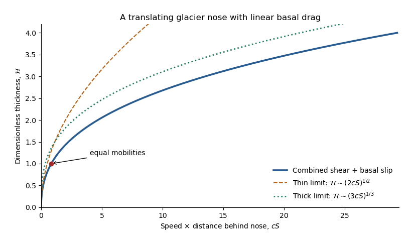
The right side is strictly increasing, giving a unique positive thickness at every $s>0$. With $S=X_N-X$ and $c=d{X}_N/d\tau$, the same relation reads $cS={\mathcal{H}}^3/3+{\mathcal{H}}^2/2$. Its limiting profiles areThe square-root tip reflects basal sliding; the cube-root thicker region reflects internal viscous deformation. Even during the early thick regime, the very nose is thin and has the square-root inner form. At late times that sliding balance governs nearly the whole profile. The dimensionless crossover thickness is $\mathcal{H}=1$ and its distance is $S=5/(6c)$; the early thick cube-root outer profile matches this smaller sliding region. The diverging geometric slope at the idealized tip also marks the local limit of the long-wave shallow-ice approximation.

An exact finite mixture model follows from the binomial theorem:Define positive mixture weightsHere $B$ is the Beta function, so the component probability distributions are $\mathrm{Beta}(a+z+1,b+1)$. All coefficients are computable from the observed integer counts.

Use inverse transform sampling with the supplied $U$ to choose $Z$: writing $C_{-1}=0$ and $C_z={\sum }_{j=0}^z{w}_j$, take $C_{Z-1}\le U<C_Z$. Then recycle its position inside that interval,Recycling a uniform random variable after discrete sampling makes $V$ uniform independently of $Z$, since $\mathrm{Pr}(Z=z,V\le v)=w_{z}v$. It is also independent of all supplied random variables with gamma distributions. Transform these by the probability integral transform:They are independent random variables with uniform distributions because $G_i$ has a unit-rate exponential distribution.

Conditional on $Z=z$, put $k=a+z+b+1$ and $r=a+z+1$. Form the $k$ values $V,W_1,\dots ,W_{k-1}$ and return their $r$th order statistic. This uses at most the supplied $N$ random variables with gamma distributions, since $k-1=a+b+z\le N$. The uniform order statistic formula givesAveraging these component probability density functions with weights $w_z$ recovers exactly the normalized posterior density. Unused inputs can be discarded. When $N=0$, $Z=0$, $k=r=1$, and the output is $U$, as required. Interval endpoints and ties have probability zero; any consistent convention there is harmless. Exactness here concerns the mathematical algorithm; finite-precision arithmetic can be stabilized with logarithmic mixture weights.

Use a genus-zero Polyakov path integral, target signature $(-,+,\dots ,+)$ and all four momenta incoming. Define the Mandelstam variables by $s=-(p_1+p_2{)}^2$, $t=-(p_1+p_3{)}^2$, $u=-(p_1+p_4{)}^2$. The string mass-shell condition is $p_i^2=4/{\alpha }^{\prime }$ and momentum conservation is ${\sum }_i{p}_i=0$, soThe reduced amplitude omits the overall momentum-conservation Dirac delta distribution and any conventional overall scattering-matrix phase. Interpret each tachyon vertex operator as normal ordered; self-contractions must not be included.

The free-boson worldsheet propagator is $⟨X^a(z)X^b(w)⟩=-({\alpha }^{\prime }/2){\eta }^{ab}\log |z-w{|}^2$. Wick theorem then evaluates the normal-ordered exponential correlator as the Koba-Nielsen factorThe worldsheet zero mode supplies momentum conservation. Four vertices give $g_s^4$ and the sphere contributes $g_s^{-2}$ through the string genus expansion, leaving $g_s^2$.

The sphere's residual Möbius transformations fix three insertion points. In sphere gauge fixing for four string vertices, take $(z_1,z_2,z_3,z_4)=(z,0,1,\infty )$. The worldsheet ghost fields, equivalently the Faddeev-Popov determinant for this residual group, supply $|z_{23}{z}_{24}{z}_{34}{|}^2$. At finite $z_4$, this determinant grows as $|z_4{|}^4$, while the matter correlator decays as $|z_4{|}^{-4}$ by momentum conservation and the tachyon mass shell; their product has a finite limit. Equivalently the weight-$(1,1)$ matter operator at infinity is normalized with $|z_4{|}^4$, while the ghost pair uses the inverse factor. After stripping the fixed-position normalization, onlyremains. Here choose the standard complex-coordinate measure $d^{2}z=idz\wedge d\bar{z}=2dxdy$. With $dxdy$ instead, the reduced normalization must acquire a factor two to give the same requested amplitude. Absolute vertex/sphere normalization is a convention; this choice fixes it consistently with the displayed $2\pi$ prefactor.

Set $a=-1-{\alpha }^{\prime }s/4$, $b=-1-{\alpha }^{\prime }t/4$, $c=-1-{\alpha }^{\prime }u/4$. Then $a+b+c=1$ and the integrand is $|z{|}^{2a-2}|1-z{|}^{2b-2}$. To evaluate the complex beta integral first work where $\mathrm{Re}a,\mathrm{Re}b,\mathrm{Re}c>0$. This ensures convergence near $0$, $1$ and infinity. Set $v=1-a$ and $w=1-b$. Schwinger parameterization givesCompleting the square, the $dxdy$ Gaussian integral is $\pi (\lambda +\rho {)}^{-1}\exp [-\lambda \rho /(\lambda +\rho )]$. Change variables to $q=\lambda +\rho$ and $x=\lambda /q$; their Jacobian determinant is $q$. Integrating $q$ gives $\Gamma (v+w-1)[x(1-x){]}^{-(v+w-1)}$. The remaining integral is the ordinary beta function $B(1-w,1-v)=B(b,a)$. ThusRestoring $d^{2}z=2dxdy$ and substituting the Mandelstam variables proves the Virasoro–Shapiro amplitude:For physical scattering the original position integral generally fails to converge. The formula defines the amplitude by analytic continuation from the convergence domain, with the desired scattering boundary value at real poles; the convergent integral should not be claimed valid for every physical momentum.

The gamma function is a meromorphic function, with simple poles at nonpositive integers and no zeros, while its reciprocal $1/\Gamma$ is an entire function. Consequently it is a meromorphic function of the independent invariants and a crossing-symmetric scattering amplitude: permuting $s,t,u$ leaves it unchanged. Its generic channel poles areand the same tower in $t$ and $u$. They represent the exchanged bosonic string mass spectrum: the tachyon, massless states including the graviton, and an infinite sequence of massive closed-string levels. There are no threshold branch cuts at this tree order.

A precise check of factorization is the Virasoro–Shapiro amplitude pole residue. Near $a=-n$, set $c=1+n-b$ in the nonsingular factor. The gamma function recurrence givesCombining this with $\Gamma (a)\sim (-1{)}^n/[n!(a+n)]$ showsThe residue is a degree-$2n$ polynomial in $t$, consistent with exchange up to spin $2n$ and scattering-amplitude factorization. At exceptional kinematics reciprocal Gamma zeros can remove apparent poles. In particular, when both $a$ and $b$ approach nonpositive integers, the zero from $1/\Gamma (a+b)$ cancels the putative double pole, leaving channel simple-pole terms. Thus one must not count products of numerator poles without using $a+b+c=1$.

Choose a branch of $t=1-z$ with $|\arg t|<\pi$ and write $d=c-a-b\notin \mathbb{Z}$. The Gauss hypergeometric equation isChanging to $t$ turns this into the same equation with third parameter $a+b+1-c=1-d$. Its solution regular at $t=0$ is $y_1=F(a,b,1-d;t)$. Substitution of $y=t^{d}v$ gives the Gauss hypergeometric equation for $v$ with parameters $c-a,c-b,1+d$. Thus $y_2=t^{d}F(c-a,c-b,1+d;t)$ is also a solution. Their distinct nonintegrally separated characteristic exponents at a regular singular point $0,d$ imply linear independence near $z=1$, soThis also follows from the exponent transformation in the Papperitz symbol.

Initially assume $\Re c>\Re b>0$, so the Euler integral for the hypergeometric function applies. If $\Re d>0$, taking $z\to 1$ gives an integral evaluated by the beta function and determinesIndeed $y_1\to 1$ and $y_2\to 0$ there. To find $B$, instead work in the nonempty parameter region $\Re d<0$, put $z=1-ϵ$ and scale the integration variable by $1-s=ϵu$. The singular contribution isThe defining integral of the beta function evaluates this integral to $\Gamma (c-b)\Gamma (-d)/\Gamma (a)$. Since ${ϵ}^{-d}{y}_1\to 0$ and ${ϵ}^{-d}{y}_2\to 1$, it determines $B$. Analytic continuation in the parameters then yields the hypergeometric connection formulaThe usual power-series definition requires $c\notin \{0,-1,-2,\dots \}$; exceptional parameters need a separately specified analytic limit. Reciprocal gamma functions make vanishing coefficients at denominator poles meaningful. The branch must remain fixed when continuing in $z$.

With the uniform prior, the binomial likelihood gives the Beta distribution posterior $\mathrm{Beta}(s+1,n-s+1)$. Under squared-error loss, the Bayes estimator is the posterior mean:

The production manager's prior gives posterior density proportional to $p^{s+1}(1-p{)}^{n-s}$. Minimizing $\mathbb{E}[(1-p)(\hat{p}-p{)}^2\mid X=s]$ gives the weighted posterior meanusing the supplied beta function. Cross multiplication shows ${\hat{p}}_P>{\hat{p}}_G$ exactly when $n>2s$, so it is greater unless $s\ge n/2$.

For $1\le k\le n$, the nearest neighbour distance ${\rho }_{(k)}(x)$ is the $k$th order statistic of $D_i=|X_i-x|$. Each $D_i$ has continuous distribution function $p_x(r)$ on $[0,\infty )$. The probability integral transform makes $U_i=p_x(D_i)$ independent and identically distributed random variables with the uniform distribution on $(0,1)$. Monotonicity of $p_x$ gives $P=U_{(k)}$, a uniform order statistic. Strict monotonicity is not needed at this stage.

For $0<s<1$, counting observations below $s$ givesDifferentiating and cancelling consecutive terms gives the Beta distribution:The Gamma function identity $\Gamma (j)=(j-1)!$ identifies this with the stated normalization. Ratios of Beta function integrals yield the momentsThis is the probability content of a nearest neighbour ball identity, specialized to intervals on the real line.

Now write $f_0=f(x)>0$. The Lipschitz bound givesThusStrict positivity of the probability density function makes $p_x$ continuous and strictly increasing from zero to one, so its inverse function is defined for every $s\in (0,1)$.

For the requested conditional calculation, suppose $f_0^2\ge L$. At $r_0=s/f_0$ the preceding bound givesTherefore $r=p_x^{-1}(s)\le s/f_0$, and substituting in the approximation proves the inverse probability content bound for a Lipschitz density:The same argument works, without $f_0^2\ge L$, on the meaningful local range $0<s<1$ with $s\le f_0^2/L$.

Since the nearest neighbour density estimator obeys $f(x)/{\hat{f}}_{(k)}(x)=2(n+1)f_0{p}_x^{-1}(P)/k$, its conditional bound follows from the Beta distribution moments:Hence, under the printed location condition,The conditional inverse function bound also bounds $p_x^{-1}(P)$, so the expected value in this calculation is finite under those formal hypotheses.