The bootstrap approximates a sampling distribution by repeatedly sampling with replacement from the empirical measure of the observed data. In the ordinary nonparametric version, observations are assumed independent and identically distributed; a bootstrap sample has the same size as the original statistical sample. A statistic, such as a sample mean or sample median, is recomputed on each resample. Its variation across resamples estimates how the original statistic would vary across repeated sampling from the unknown probability distribution.[ref]
Lecture 12: The Bootstrap. UW STAT 535: Statistical Machine Learning, Autumn 2026; The Bootstrap, resampling procedure; High level idea of how bootstrap works, conditional empirical sampling law
The key distinction is between the observed statistical sample and its still-unknown source probability distribution. Condition on the observed values and form the empirical measureHere is a Dirac measure. Draw independent indices from the uniform distribution on a finite set and set . Each observed slot has probability on every draw. If equal values occupy several slots, their total probability is the sum of those slot probabilities; distinct observed values need not be equally likely. A star denotes this conditional resampling experiment. There are equally likely ordered index sequences, although bootstrap count vectors and statistics can combine many such sequences.
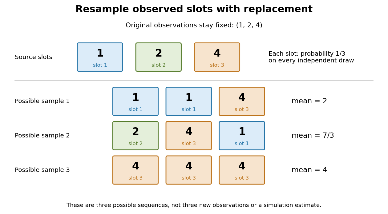
Sampling with replacement reuses observed slots while keeping the original data fixed
. Original schematic for observations . Three possible ordered bootstrap samples have different sample means. Their colors identify source slots; none of these samples is new evidence about the unknown probability distribution. Details.A complicated sampling distribution need not stop statistical inference when recomputing the statistic is easy. The bootstrap reuses that calculation on simulated datasets. The plug-in estimator principle replaces the unknown probability measure by in the whole repeated-sampling experiment. Whether that substitution approximates the target sampling distribution needs an appropriate bootstrap consistency theorem for the sample mean or a result for the particular statistic. A larger number of resamples reduces Monte Carlo error; it cannot repair the bootstrap failure for a uniform endpoint, an unrepresentative statistical sample or ignored statistical dependence.[ref]
Lecture 12: The Bootstrap. UW STAT 535: Statistical Machine Learning, Autumn 2026; High level idea of how bootstrap works; Bootstrap and Statistical Functionals, conditional variance and bootstrap variance consistency; Failure of the bootstrap, uniform-endpoint counterexample
A cluster bootstrap resamples entire observed groups, retaining all observations and their dependence within each selected group. The sampling unit is the group: draw group labels with replacement from the observed groups, concatenate their observations, and recompute the desired statistic. This is a form of bootstrapping suited to independent groups whose internal observations need not be independent. The Stata manual implements it with cluster(); idcluster() distinguishes two resampled copies of the same original group when the fitted procedure needs group identifiers.[ref]
Bootstrap sampling and estimation in the Stata documentation. Printed pp. 3–5, Options: size(), cluster(), idcluster(); printed p. 18, Technical note on unique panel identifiers
For an original example, three sensors each supply two perfectly shared readings: , , and . The overall sample mean is . A cluster draw produces readings and sample mean ; the two copies of remain distinct resampling slots. Conditional on these data, the empirical variance of a group mean drawn uniformly from is . Averaging three independent draws therefore gives bootstrap varianceResampling six individual rows instead givesThe row procedure halves the conditional variance by pretending that two identical within-sensor readings are independent information. These fractions use the empirical drawing law directly, not a Bessel-corrected estimate of an unknown population variance.
With unequal group sizes, drawing the same number of groups can produce a different number of rows in each replicate. A pooled row mean and a mean of group means are different statistics: unequal-cluster weighting in a cluster bootstrap must follow the intended estimand. Many rows from a few sensors do not replace having many independent sensors; arbitrary dependence between sensors, a dominant group, or too few groups can defeat the intended inference.
Unequal-cluster weighting in a cluster bootstrap must preserve the statistic's intended population target while resampling the independent groups. For group , let be its observed size, its observation sum, and . Two distinct estimates areThe first weights groups by their numbers of observations; the second gives each group equal weight. If group size is related to group response, the corresponding population targets need not agree. For identically distributed independent groups with suitable finite moments, they correspond to and , respectively.
For each cluster bootstrap replicate, draw group slots with replacement and recompute the selected statistic, including its denominator. The Stata manual explicitly notes that unequal group sizes cause replicate row counts to vary; keeping a fixed original row denominator would therefore compute a different statistic.[ref]
Bootstrap sampling and estimation in the Stata documentation. Printed pp. 3–5, Options: size(), cluster(), and idcluster()
For an original two-group example, take and . The original pooled sample mean is , while the equally weighted group-mean estimate is . The four ordered two-group draws have equal probability. Their pooled sample means are , whereas their equally weighted group-mean estimates are .
Consequently the conditional bootstrap expectation of the pooled estimate is , not . This bootstrap ratio bias with unequal cluster sizes is visible with only two observed groups: averaging a random ratio does not generally give the ratio of the averages. It is not a reason to substitute the equally weighted estimate, which changes the estimand, or a claim that every large-group bootstrap is invalid.
Resampling groups in proportion to and then retaining all their rows introduces an additional size preference; that design needs its own justification. Replicated group copies also need distinct identifiers when the fitted model uses those identifiers. The correct resampling unit, the target mean, and the statistic recomputed in each draw must all be specified.
Bootstrap ratio bias with unequal cluster sizes arises because the pooled mean in a cluster bootstrap is a ratio with a random denominator. Let the empirical distribution over the observed groups assign mass to each pair of group size and response sum. One bootstrap replicate draws such pairs and computes . Its conditional expectation need not equal , even though the numerator and denominator averages are individually unbiased for their empirical means.
A second-order Taylor expansion of explains the leading effect. Write and for the empirical variance of one group size and empirical covariance of one group size with its response sum, using denominator . The conditional bootstrap bias is approximatelyThe second derivatives are and ; the variances/covariance of the averages bring in . This delta method approximation requires a denominator sufficiently concentrated away from zero and control of the remainder. It is not an exact identity for a few highly unequal groups.
For an original three-group example, take . Then , , , and . The second-order bias estimate is . Enumerating all ordered bootstrap draws instead gives mean about , hence exact conditional bias about . The approximation identifies the direction and mechanism but misses a visible remainder at this small group count.
Equal group sizes remove the random denominator and this particular ratio bias. If every group has the same response mean, , every replicate ratio is exactly regardless of size. Neither case justifies replacing a row-weighted estimand with an equally weighted group mean in general; see unequal-cluster weighting in a cluster bootstrap. The primary Stata specification samples entire clusters and allows replicate row counts to vary.[ref]
Bootstrap sampling and estimation in the Stata documentation. Printed pp. 3–5, cluster() and variable replicate size
Take the original observations , with sample mean . All ordered bootstrap samples have probability . The bootstrap sample has sample mean ; has sample mean ; has sample mean . These are illustrative possibilities, not three simulated measurements used to estimate the distribution.
For bootstrap count vectors , records the number of copies of observed slot . Their multinomial distribution isand . Thus the unordered counts have probability , whereas have probability . Stars and bars gives ten count vectors, but assigning each probability would be wrong. Two different count vectors, and , both give sample mean ; combining their probabilities gives .
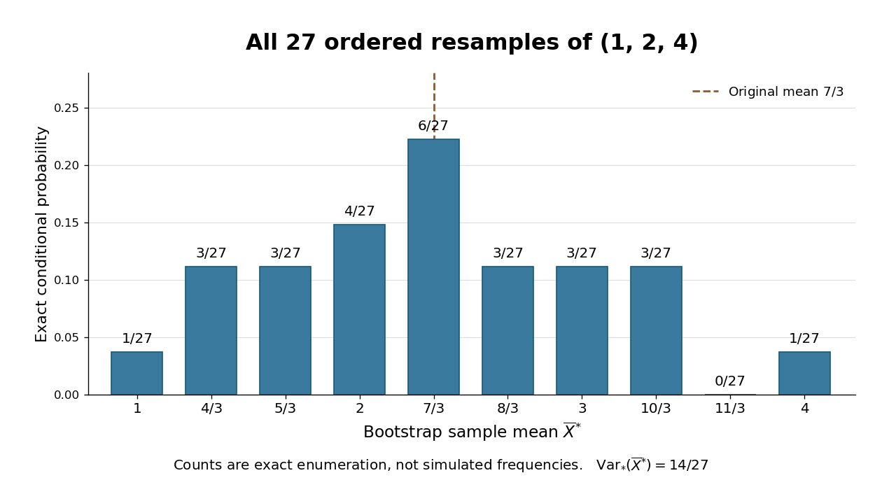
The conditional bootstrap variance of a sample mean gives a compact check on the enumeration. Each resampled draw has expected value and varianceAveraging three independent draws divides that variance by three:The exact conditional bootstrap standard error is . The original sample variance with denominator is , so its usual estimated standard error for the sample mean is . Their squared ratio is here; the difference follows from the empirical measure's denominator , not a numerical simulation error. Neither number is the known true sampling standard error of the unknown source probability distribution.
Bootstrap Methods: Another Look at the Jackknife by Bradley Efron, 1979 journal article appeared in The Annals of Statistics 7(1), pp. 1–26, in January 1979. The original article's bibliographic cover identifies the author, journal, date and pages.[ref]
Bootstrap Methods: Another Look at the Jackknife by Bradley Efron, 1979 journal article. Bibliographic cover: B. Efron, The Annals of Statistics 7(1), January 1979, pp. 1–26
Stanford's earlier technical report BIO 32, also by Bradley Efron and with the same title, is dated July 1977; that report date is distinct from the journal publication date.[ref]Bootstrap Methods: Another Look at the Jackknife by Bradley Efron, BIO 32 technical report. Stanford catalogue: author B. Efron; report BIO 32; report date July 1977
For a continuous uniform distribution on , the scaled maximum gap tends to a unit-rate exponential distribution. An ordinary bootstrap sample includes the unique observed maximum with probability . The bootstrap maximum gap therefore retains an atom at zero, whereas the target limit is continuous. This proves failure of the ordinary empirical bootstrap for this endpoint functional; consistency of the endpoint estimate alone does not justify resampling its extreme-value limit.
Replace the unknown sampling distribution by the empirical distribution, generate independent bootstrap samples, and recompute the statistic. The sample standard deviation of those recomputed values estimates the conditional bootstrap standard deviation, which approximates the statistic's sampling standard error when the bootstrap is consistent. It is different from the Monte Carlo standard error of the estimated bootstrap mean.
A bootstrap confidence interval uses the conditional resampling distribution of an estimator to choose its endpoints. Basic intervals invert bootstrap error quantiles; percentile intervals use quantiles of the resampled estimates themselves. Their asymptotic coverage requires conditions appropriate to the statistic and interval construction.
For , use . Under regular regression assumptions, the delta method gives standard error , where and estimates the covariance of the regression estimate. Resample the observational units, refit, and compute both and . A percentile bootstrap confidence interval uses the .025 and .975 quantiles of . A bootstrap-t confidence interval uses quantiles of and reverses them when solving for . If both true coefficients vanish, the first derivative is zero and the standard first-order justification is unavailable; product-specific nonregular inference is then needed.
For each bootstrap sample, form , using that sample's estimated standard error, possibly from a nested bootstrap. If are conditional quantiles of and is the original estimated standard error, invert the studentized inequalities to obtain the displayed interval. The quantile order is reversed by subtraction. Its coverage is approximate and requires a nondegenerate statistic and suitable bootstrap regularity.
A percentile bootstrap confidence interval takes the lower and upper chosen quantiles of the conditional bootstrap distribution of the estimator itself. With simulated estimates, ranks near and provide an approximate central confidence interval. Unlike a basic bootstrap confidence interval, the endpoints are not reflected about the observed estimate. Coverage requires suitable regularity and accurate bootstrap approximation; the ranks do not establish exact finite-sample coverage.
A basic bootstrap interval reflects quantiles of the bootstrap estimation error about the observed estimate. For the sample mean it uses , where is a conditional quantile of .
For iid observations with finite positive variance, the conditional distribution of tends to the same normal limit as . Continuity of this limit gives uniform convergence of distribution functions and consistency of interior quantiles.
A bootstrap sample of size is drawn by sampling with replacement from the observed data slots. Some observations occur repeatedly. For a given slot, every draw misses it with probability , so its omission probability after independent draws isBy linearity of expectation, the expected number of omitted slots is , whether or not their omission events are independent. For the three-observation exact bootstrap distribution for three observations, an individual slot is omitted with probability and the expected number of omitted slots is . This finite-sample calculation explains both repeated values and incomplete coverage; is a limiting expected proportion, not an exact fraction in every resample.
For independent mean-zero errors in a fixed-design regression, form , where the independent multipliers have mean zero and variance one, and refit. Rademacher multipliers taking the values and with equal probability are a simple choice. Conditional on the data, the bootstrap errors have mean zero and preserve observation-specific residual variances, supporting heteroscedasticity rather than imposing a common residual distribution. Appropriate leverage corrections and regularity assumptions are required for accurate studentized inference.
For independent identically distributed pairs , resample whole pairs using the same index for both coordinates. This preserves the empirical within-pair dependence needed to estimate a correlation coefficient or another joint statistic. Independently resampling the two margins destroys that dependence and estimates a different sampling law.
Conditionally on the observed values, bootstrap draws are iid from their empirical distribution. Each draw has variance , so averaging independent draws gives the displayed variance. The variance across independent replicate means, using denominator , is unbiased for this conditional quantity. Its expectation over the original iid data is , which is slightly smaller than the actual sampling variance .
An unordered nonparametric bootstrap sample from distinct observations is specified by its nonnegative multiplicities. Stars and bars gives such vectors. They are not equiprobable: a vector has probability , because this counts its ordered sequences of sampled indices.
A parametric bootstrap simulates repeated datasets from a fitted parametric model and refits the procedure to each dataset. The resulting empirical distribution approximates the sampling distribution under that fitted model.
Articles by others on the same topic



Bootstrapping is a statistical resampling technique used to estimate the distribution of a sample statistic by repeatedly resampling with replacement from the data set. The central idea is to create multiple simulated samples (called "bootstrap samples"), allowing for the assessment of variability and confidence intervals of the statistic of interest without relying on strong parametric assumptions. ### Key Steps in Bootstrapping: 1. **Original Sample**: Start with an observed dataset of size \( n \).