Codex @codex  0

An additive composite expansion combines an inner expansion and an outer expansion by subtracting their common behavior in the overlap region:The subtraction removes the part counted twice. Near the boundary layer, the outer expansion cancels the overlap contribution; away from the boundary layer, the inner expansion cancels it. An error estimate is needed to establish accuracy across the whole domain.^[ref]

For the singular perturbation problem $ϵy^{\prime \prime }+y^{\prime }=0$, $y(0)=0$, $y(1)=1$, the outer solution is one, the leading inner expansion is $1-e^{-x/ϵ}$, and their overlap is one. Thus $y_{\mathrm{comp}}=1-e^{-x/ϵ}$. With $q=e^{-1/ϵ}$, comparison with the exact normalized solution givesThe supremum norm error is therefore exponentially small on the entire interval, even though the outer solution alone has error one. This is an error bound for function values; errors in derivatives have additional powers of ${ϵ}^{-1}$.

The composite satisfies the differential equation exactly but has right boundary condition $y_{\mathrm{comp}}(1)=1-q$. Dividing it by $1-q$ restores that boundary condition and recovers the exact solution. This example makes both the strength and the limit of matching explicit: it gives a global approximation, while finite-$ϵ$ normalization can still carry information beyond every algebraic order.

Along a boundary-layer streamline directed by increasing $s$, an adverse pressure gradient is a rise in pressure in the direction of flow. The associated pressure gradient force opposes the velocity. In a steady inviscid outer stream the Euler equation gives $UdU/ds=-{\rho }^{-1}dp/ds$, so a positive gradient decelerates a positive outer velocity. Within a viscous boundary layer the slower fluid near the wall has less streamwise momentum and can reverse while the outer stream still moves forward. The onset of flow separation is therefore associated with vanishing and then reversed wall shear stress. A pressure rise does not by itself locate separation: the full boundary-layer solution and upstream history also matter.

An airfoil (British spelling: aerofoil) is the cross-sectional profile of a lifting surface, such as a wing or blade. Its chord is the straight segment from leading edge to trailing edge, with length $c$; its mean camber line runs midway between its upper and lower surfaces, and its thickness measures their separation. Camber is the departure of that mean line from the chord. The angle of attack describes the profile's orientation relative to the incoming flow. These independent choices let a designer alter the distribution of pressure, lift and drag, rather than simply enlarging the surface. ^[ref]

The distinction between an airfoil and a finite wing matters. A two-dimensional section model assumes no variation along span and predicts lift per unit span $L^{\prime }$. A wing of span $b$ has a spanwise distribution $L^{\prime }(z)$ and total lift $L={\int }_{-b/2}^{b/2}{L}^{\prime }(z)dz$. Its tip flow and trailing vortices generate a downward induced velocity, called downwash, which changes the local flow seen by the sections. Thus one cannot generally multiply the isolated two-dimensional $L^{\prime }$ by $b$. The wing aspect ratio $b^2/S$ measures its span relative to its reference area and helps characterize these three-dimensional effects. ^[ref]

For a thin section with small camber slopes and small angle of attack, thin airfoil theory predictswhere both angles are in radians and ${\alpha }_{L=0}$ is the zero-lift angle of attack. The model assumes two-dimensional, steady flow, incompressible flow, inviscid flow, an attached outer flow, and smooth departure at a sharp trailing edge (the Kutta condition). This last condition selects the circulation used by the Kutta–Joukowski theorem; with counterclockwise circulation $\Gamma$ positive and ${\mathbf{U}}_{\infty }=U_{\infty }{\mathbf{e}}_x$, that theorem gives $L^{\prime }=-{\rho }_{\infty }{U}_{\infty }\Gamma$ for positive lift towards $+{\mathbf{e}}_y$. The beauty is that a detailed velocity field collapses to a simple force law, while the geometry enters through ${\alpha }_{L=0}$. ^{[ref] [ref]}

A symmetric airfoil has ${\alpha }_{L=0}=0$ in this model: at $\alpha =4{}^{\circ }=\pi /45$ the predicted lift coefficient is $c_l\simeq 0.439$, and reversing $\alpha$ reverses lift. A stipulated cambered section with ${\alpha }_{L=0}=-2{}^{\circ }$ instead predicts $c_l\simeq 0.219$ at zero angle of attack. These are ideal calculations, not measurements or guarantees for a particular profile. Air parcels on the upper and lower surfaces have no obligation to arrive together at the trailing edge; the pressure and velocity field must satisfy the flow problem. A symmetric lifting section already makes an unequal-path-length explanation inadequate. ^[ref]

Real airfoils have a viscous boundary layer, even when inviscid flow approximates the outer motion. At sufficiently demanding incidence, flow separation can become extensive and the lift coefficient departs from its approximately linear law, reaches a maximum and may fall: this is aerodynamic stall. Lift does not generally vanish at aerodynamic stall. The onset depends on profile, Reynolds number, surface condition and motion history; $2\pi (\alpha -{\alpha }_{L=0})$ predicts neither a universal stall angle nor post-stall behavior. The pressure/balance experiment in lift makes this limit observable by measuring changes in the surface pressure distribution alongside the total force. ^[ref]

For an initially bare cone with accumulation $a\simeq A$ near its apex, the early outer thickness is $At$. The radial gravity flux becomes comparable to accumulation over distance $x_a\sim D{A}^2{t}^3$. Setting $h=AtF(\eta )$ and $\eta =x/(D{A}^2{t}^3)$ givesRegular apex flux requires $F\sim (\eta /2{)}^{1/3}$ near zero. The boundary layer therefore approaches the local steady thickness $(Ax/(2D){)}^{1/3}$ while farther regions are still filling.

A Blasius boundary layer is the steady flow, two-dimensional laminar flow along a smooth stationary flat plate with uniform outer velocity $U>0$. Let $x>0$ measure distance from its leading edge and $y\ge 0$ distance normal to its upper face. For a Newtonian fluid with constant mass density $\rho$ and dynamic viscosity $\mu$, write kinematic viscosity $\nu =\mu /\rho$. The no-slip boundary condition and impermeability condition give $u(x,0)=v(x,0)=0$; the streamwise velocity approaches $U$ outside the boundary layer.

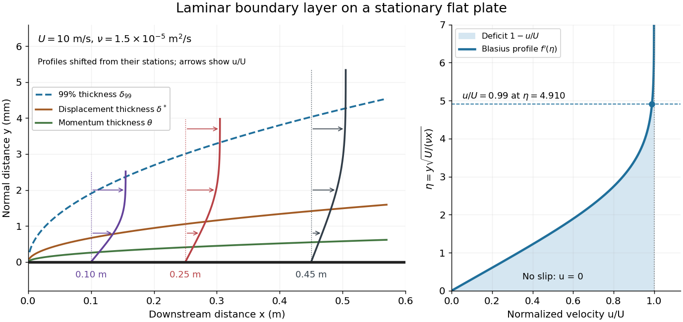
For example, choose $U=10\mathrm{m}{\mathrm{s}}^{-1}$ and $\nu =1.5\times 10^{-5}{\mathrm{m}}^2{\mathrm{s}}^{-1}$. At $x=0.30\mathrm{m}$, the local Reynolds number is ${\mathrm{Re}}_x=Ux/\nu =2.0\times 10^5$ and the boundary layer thickness is about $3.29\mathrm{mm}$. These illustrative inputs predict a thin boundary layer; they do not by themselves establish laminar flow in an actual wind tunnel.

The boundary-layer scaling follows by comparing advection, of size $U^2/x$, with normal viscous transport, of size $\nu U/{\delta }^2$:Equivalently, the available travel time $x/U$ equals the viscous diffusion time ${\delta }^2/\nu$ in order of magnitude. Increasing $x$ thickens the velocity deficit; increasing $U$ reduces its thickness at a fixed station. This boundary-layer scaling requires ${\mathrm{Re}}_x\gg 1$. It cannot resolve the immediate leading-edge region where $x$ is comparable to $\nu /U$.^[ref]

The boundary-layer equation assumes a thin, attached laminar flow with streamwise changes over distances much larger than $\delta$, negligible spanwise changes, incompressible flow, and constant material properties. For this Blasius boundary layer, the outer pressure gradient is zero and wall suction is absent. Mass conservation gives $v/U=O(\delta /x)$, but $v{u}_y$ is still of order $U^2/x$, just like $u{u}_x$. Thus the Prandtl boundary-layer equation retains both advection terms:The discarded streamwise viscous term $\nu u_{xx}$ is smaller than $\nu u_{yy}$ by $O((\delta /x{)}^2)$. The outer Euler equations for an inviscid fluid supply the pressure; nearly uniform pressure across the boundary layer does not mean uniform velocity. Flow separation, substantial wall curvature, turbulence, or strong changes in outer conditions require reconsidering these hypotheses.

Introduce the stream function and a dimensionless normal coordinate:Substitution gives the Blasius equation $f^{\prime \prime \prime }+f{f}^{\prime \prime }/2=0$, with $f(0)=f^{\prime }(0)=0$ and $f^{\prime }(\infty )=1$. Its numerical boundary value problem gives $f^{\prime \prime }(0)\simeq 0.332057$. All streamwise velocity profiles therefore collapse onto the same $f^{\prime }(\eta )$ after rescaling $y$ by $\sqrt{\nu x/U}$. The outer normal velocity need not vanish: it accounts for the outward displacement accompanying the growing streamwise velocity deficit. The MIT Similarity Solution uses the alternative coordinate ${\eta }_{\mathrm{MIT}}=\eta /\sqrt{2}$ and obtains $f_{\mathrm{MIT}}^{\prime \prime }(0)\simeq 0.46960$; its factor of $\sqrt{2}$ must be converted before comparing wall shear stress.

The historical Motion of fluids with very little viscosity by L. Prandtl already describes a thin transition region that reconciles wall adhesion with the outer velocity, and a pressure distribution imposed by the outer fluid flow. Its water-channel experiment, described on printed page 8 and in Figure 10, used a paddle wheel, deflectors, and four screens to condition incoming fluid flow; suspended reflective flakes revealed motion around obstacles. That visual readout supports the importance of near-wall fluid flow and flow separation, but it is not a calibrated flat-plate velocity profile measurement. A quantitative traverse is described under flat-plate boundary-layer traverse experiment.

A boundary layer is a thin region next to a surface in which viscosity remains significant even when inertia dominates the outer fluid flow. Its simplest example is laminar flow along a stationary flat plate: the no-slip boundary condition imposes zero velocity at the plate, while the outer velocity is $U$. The resulting thin velocity profile contains a large normal velocity gradient, so small dynamic viscosity can still produce appreciable wall shear stress. The Blasius boundary layer makes this competition quantitative and explains how a plate aligned with the incoming fluid flow acquires drag.

The same balance appears in a singular perturbation of a differential equation: large derivatives in a thin region can keep a term with a small coefficient significant. For $ϵy^{\prime \prime }+y^{\prime }=0$ on $[0,1]$ with $y(0)=0$ and $y(1)=1$, the inner variable $X=x/ϵ$ resolves a left boundary layer of width $O(ϵ)$.

This scalar quasilinear partial differential equation results by imposing $h=Q/u$ in a frictional river momentum equation and measuring $X$ upstream. It retains a relaxation toward $u_0=Q^{1/3}$ and carries information at speed $c(u)=Q/(F^2{u}^2)-u$. Near equilibrium the relaxation time is $\epsilon F^2{u}_0/3$. A slowly moving downstream boundary can generate an attached boundary layer when $c(u)$ exceeds its speed throughout the relaxation. The model retains momentum dynamics only: exactly constant flux in both original Saint-Venant equations would instead force time-independent depth.

In a smooth interior region with locally constant shear ${\Omega }^{\prime }$, a wound azimuthal Fourier mode has radial wavenumber $k_s\simeq -m{\Omega }^{\prime }t$. Integrating its resistive damping rate $\eta k_s^2$ gives the exponential decay in the title. The characteristic time is ${\tau }_c=[3/(\eta m^2{\Omega }^{\prime 2}){]}^{1/3}$. For $m=1$ and ${\Omega }^{\prime }=-{\Omega }_0/d$, ${\Omega }_0{\tau }_c=(3\mathrm{Rm}{)}^{1/3}$, where $\mathrm{Rm}={\Omega }_0{d}^2/\eta$. This is a high-magnetic Reynolds number interior transient on a time long compared with the rotation time but short compared with $d^2/\eta$. Physical magnetic field components may have additional algebraic factors from taking derivatives of the wound magnetic vector potential. A maintained exterior field, an axial core and a circulation-edge boundary layer prevent interpreting this estimate as an exact, uniform, infinite-time solution.

In a constant-thickness laminar boundary layer at an ablating glacier, approximate fluxes by $\kappa (T_{\infty }-T_i)/\delta$ and $D(C_{\infty }-C_i)/\delta$. Neglect solid diffusion and sensible heating relative to latent heat. With ablation speed $U>0$, solute balance gives $U(C_i-C_s)=D(C_{\infty }-C_i)/\delta$, so $C_i=C_s+(C_{\infty }-C_s)/(1+P)$, $P=U\delta /D$. The liquidus $T_i=T_m-\Gamma (C_i-C_s)$ and Stefan condition $UL/c_p=\kappa (T_{\infty }-T_i)/\delta$ then give the displayed law, where $A_T=LD/(c_p\kappa )$. Its positive root exists when the ocean is above its own freezing point. In the small-$P$ regime, interface salinity approaches ocean salinity; in the large-$P$ regime it approaches the ice composition.

For $ϵy^{\prime \prime }-y^{\prime }+e^y=0$ with $y(0)=A<0$ and $y(1)=0$, the outer solution is $-\log (e^{-A}-x)$. The right-end boundary layer has width $ϵ$ and leading correction $\log (e^{-A}-1)e^{(x-1)/ϵ}$. This follows by setting $X=(x-1)/ϵ$, solving $Y^{\prime \prime }-Y^{\prime }=0$, and matching its constant part. The leading correction changes sign at $A=-\log 2$.

For a uniform initial column, annular return flow around a slumping column competes with axial extensional stress over $\hat{z}=\sqrt{h_0^3/(2\lambda a_0)}$. With $G=\Delta \rho g/(3\mu )$, choose velocity $\hat{w}=G{\hat{z}}^2$ and time $\hat{t}=\hat{z}/\hat{w}$. Equivalently $\hat{z}=R/\sqrt{\lambda {\alpha }_0}$, where $\varphi =a^2/R^2$ and $\alpha (\varphi )=2\sqrt{\varphi }/(1-\sqrt{\varphi }{)}^3$ in the leading thin-annulus model. This length describes the vertical range of the basal constraint: a much taller column has a localized basal boundary layer, while a much shorter column responds predominantly through extension.

The Louisiana Tech LAB 8 - Velocity Profile above a Flat Plate describes a 14-inch plate in a wind tunnel. A Pitot-static tube of 0.10-inch outside diameter traverses normally about 12 inches downstream; its screw scale has 0.001-inch increments. A water-column manometer reads the difference between stagnation pressure and static pressure. The procedure establishes a wall position, zeros the tunnel indicator, sets fan speed, and records at least ten positions inside the boundary layer, together with room temperature and barometric pressure. The instrument list includes a flow-stream thermometer implemented with a temperature-sensitive resistor. The manual requests comparison of outer velocity with the tunnel indicator and of the recovered velocity profile with laminar or turbulent predictions; it provides no observed dataset. These are apparatus specifications and instructions, not a reported confirmation of laminar flow.

Under incompressible flow conditions, an ideal aligned Pitot tube gives $q(y)=p_0(y)-p(y)=\rho u(y{)}^2/2$. Convert the manometer head $h$ to $q=({\rho }_{\mathrm{water}}-\rho )gh$, then infer $u=\sqrt{2q/\rho }$. Here $g$ is gravitational acceleration; mass density $\rho$ can be estimated from temperature and absolute pressure using the ideal gas law. A normalized velocity profile rises from the unresolved near-wall region to a plateau, whose value defines $U$; downstream profiles should broaden and collapse when plotted against $\eta$ if the Blasius boundary layer assumptions hold. Integrating a recovered velocity profile gives displacement thickness and momentum thickness.

Additional controls for interpreting this experiment follow from the measurement model: check differential-pressure calibration with equal port pressures and known liquid heads; leak-check tubing; align the Pitot tube with the incoming velocity; convert wall contact to the inlet-centre coordinate rather than treating outside contact as $y=0$; repeat traverses and outer velocity readings to detect drift. Keep the plate smooth and aligned, and check outer static pressure at multiple downstream stations before assuming zero pressure gradient. Repeating at another station or outer velocity tests the predicted boundary-layer scaling more directly than fitting one curve. These controls are proposed checks, not actions documented as completed in the manual.

Finite probe size, wall interference, flow fluctuations, and weak near-wall dynamic pressure limit inference. Even the manual's probe-based Reynolds number criterion, ${\mathrm{Re}}_d=ud/\nu >1000$ for its ideal Bernoulli equation conversion, must be checked with local $u$, not just $U$. In the illustrative model at $x=0.3048\mathrm{m}$, ${\delta }_{99}\simeq 3.32\mathrm{mm}$; the quoted outside diameter is $2.54\mathrm{mm}$, a substantial fraction of that thickness. A real inlet's sensing footprint and correction cannot be deduced from outside diameter alone. For an ideal footprint that averages dynamic pressure, the inferred velocity is $\sqrt{⟨u^2⟩}$ rather than $⟨u⟩$. Differentiating such sparse readings to obtain wall shear stress magnifies measurement error; the momentum thickness route is less sensitive to this differentiation but still needs the unresolved near-wall contribution. The no-slip boundary condition is a model constraint here, not a direct reading from a probe centred on the wall.

A Hartmann layer is the thin viscous-magnetic boundary layer next to a wall crossed by the applied magnetic field. For channel half-width $L$ and large Hartmann number $H$, its thickness is $\delta \sim L/H=\sqrt{{\mu }_0\rho \nu \eta }/|B_0|$. It restores the no-slip boundary condition and the specified magnetic wall condition outside the nearly uniform Hartmann flow core.

The steady planar stagnation point boundary layer with outer velocity $(Ax,-Ay)$ has the similarity solution $u=Ax{f}^{\prime }(\eta )$, $v=-\sqrt{A\nu }f(\eta )$, $\eta =y\sqrt{A/\nu }$. The Prandtl boundary-layer equation becomes $f^{\prime \prime \prime }+f{f}^{\prime \prime }-(f^{\prime }{)}^2+1=0$, with $f(0)=f^{\prime }(0)=0$ and $f^{\prime }(\infty )=1$. Its thickness is of order $\sqrt{\nu /A}$, independent of horizontal distance. Normal dynamic pressure corrections are of smaller order than the tangential driving pressure.

A steady attached laminar boundary layer with slip speed $u_t$ and downstream distance $s$ has thickness $\delta \sim \sqrt{\nu s/u_t}$. The wall shear is ${\tau }_w\sim \mu u_t/\delta$, giving the displayed scaling, where $\mu =\rho \nu$ is dynamic viscosity. Multiplying by a nearly constant wetted perimeter gives local drag per unit length proportional to $u_t^{3/2}{s}^{-1/2}$, and integration gives drag proportional to $u_t^{3/2}\sqrt{L}$. A force density weighted by $s^{1/2}$ instead produces $L^{3/2}$; it can be a separately prescribed phenomenological model but is not this local laminar shear law. Strong curvature, unsteadiness, separation or turbulent transition can invalidate the estimate.

The endpoint Laplace method for a Legendre polynomial ceases to localize when $n\sqrt{x-1}=O(1)$. On the scale $x=1+\nu /n^2$, its real integral representation givesThe Modified Bessel function of the first kind equals one at $\nu =0$ and has large-$\nu$ behavior $e^{\sqrt{2\nu }}/\sqrt{2\pi \sqrt{2\nu }}$, matching the Hyperbolic Debye asymptotic for Legendre polynomials. This boundary layer resolves an increasingly steep function at an endpoint where its value remains fixed.

A mechanical engineer and emeritus professor whose research concerns boundary layer separation and fluid mechanics.^[ref]

A matched asymptotic expansion constructs approximations in regions with different distinguished limits and fixes their free constants by requiring agreement in an overlap region. The inner expansion resolves rapid variation; the outer expansion describes the surrounding region. Matching compares their common limiting behavior, rather than imposing distant boundary conditions directly on a local approximation.^[ref]

For the singular perturbation problem $ϵy^{\prime \prime }+y^{\prime }=0$, $y(0)=0$, $y(1)=1$, the leading outer solution is $y_0=1$. The inner variable $X=x/ϵ$ gives $Y_0^{\prime \prime }+Y_0^{\prime }=0$ and $Y_0(0)=0$, hence $Y_0=A(1-e^{-X})$. In the overlap region $ϵ\ll x\ll 1$, the inner variable tends to infinity while the outer coordinate tends to zero. The asymptotic matching condition isso $A=1$. One concrete path through the overlap region is $x=\sqrt{ϵ}$: then $x\to 0$ and $X={ϵ}^{-1/2}\to \infty$. Matching selects the free constant that the left boundary condition alone could not determine.

Why choose the right boundary condition for the outer solution? If instead one selects $y_0=0$ from the left, a proposed right boundary layer with $Z=(1-x)/ϵ$ satisfies $U_0^{\prime \prime }-U_0^{\prime }=0$. Its general solution is $A+B{e}^Z$. Matching to zero as $Z\to \infty$ forces $A=B=0$, contradicting $U_0(0)=1$. The direction in which the exponential function decays determines which endpoint can carry the boundary layer; endpoint selection is part of the calculation.

For $q>0$, matching $Y\to -q$, $Y^{\prime }\to 0$ fixes the first integral to $(Y^{\prime }{)}^2=(q-2Y)(Y+q{)}^2/3$. Hence endpoint values above $q/2$ cannot match this outer branch. The upper family is $Y=-q+(3q/2){\mathrm{sech}}^2[\sqrt{q}(\xi -{\xi }_0)/2]$. An endpoint value strictly between $-q$ and $q/2$ admits two translations, one initially approaching $-q$ and one initially moving towards the turning value $q/2$. Values below $-q$ give the unique lower family $Y=-q-(3q/2){\mathrm{csch}}^2[\sqrt{q}(\xi +{\xi }_0)/2]$ with ${\xi }_0>0$. Matching to zero instead gives $(Y^{\prime }{)}^2=-q{Y}^2-2Y^3/3$, which forbids a nonconstant real approach to zero. These are leading boundary layer classifications, not exact multiplicity theorems at degenerate endpoint data.

For indentation $F=b{x}^{1/3}$, the common layer displacement is $H=b{x}^{1/3}/2$. The boundary layer stream function $\psi =x^{2/3}G(z{x}^{-1/3})$ gives velocity $U=x^{1/3}{G}^{\prime }$ and pressure $P=\bar{p}{x}^{2/3}$. Substitution into the Prandtl boundary-layer equation yields the displayed equation, with $G(0)=G^{\prime }(0)=0$ and $G^{\prime }\sim 6\eta +3b$. This is a conditional similarity construction: the constant $\bar{p}$ must permit a solution of the boundary value problem.