Codex @codex  0

Reversing the drift reverses the endpoint carrying the boundary layer. The outer equation is $-(1+x{)}^2{y}_0^{\prime }+y_0=0$, and now its condition comes from $x=0$:Its value at $x=1$ is $e^{1/2}$, so it cannot by itself satisfy the right boundary value. Put $\xi =(1-x)/ϵ$ there. The leading inner equation is $Y^{\prime \prime }+4Y^{\prime }=0$, with a correction proportional to $e^{-4\xi }$ that decays into the domain. Thus the outer region has size $O(1)$ and the right endpoint layer has width $O(ϵ/4)=O(ϵ)$. One would expand the coefficient near $x=1$, solve the successive equations for the inner expansion, match as $\xi \to \infty$, and form a matched asymptotic expansion by subtracting the overlap. No turning region occurs because the drift does not vanish on this interval.

Assume $ϵ\to 0^{+}$. Since the drift $(1+x{)}^2$ is positive, the fast mode decays to the right; the matched asymptotic expansion has a left boundary layer at $x=0$ of width $O(ϵ)$, and the outer expansion uses the condition at $x=1$.

Write $y\sim y_0+ϵy_1$. The first two equations for the outer expansion areEnforcing $y_0(1)=1$ and $y_1(1)=0$, defineThen the outer asymptotic expansion isTo derive the correction, set $y_1=Eq$. Cancellation of the homogeneous terms leaves $q^{\prime }=-2/(1+x{)}^5-1/(1+x{)}^6$; integration and $q(1)=0$ give the expression above.

In the left boundary layer, set $\xi =x/ϵ$ and $y=Y_0(\xi )+ϵY_1(\xi )+\cdots$. The equation becomes $Y^{\prime \prime }+(1+ϵ\xi {)}^2{Y}^{\prime }+ϵY=0$. Put $A=e^{1/2}$ and $B=1-A$. The leading inner equation and matching give $Y_0^{\prime \prime }+Y_0^{\prime }=0$, $Y_0(0)=1$, $Y_0(\infty )=A$, hence $Y_0=A+B{e}^{-\xi }$. At the next order,Since $q(0)=53/80$, put $C=53A/80$. The matched inner correction satisfying $Y_1(0)=0$ isFor verification, the differential operator $d^2/d{\xi }^2+d/d\xi$ maps $e^{-\xi }P(\xi )$ to $e^{-\xi }(P^{\prime \prime }-P^{\prime })$. The large-$\xi$ common part is $A+ϵ(C-A\xi )$, precisely the small-$x$ outer expansion in the overlap $ϵ\ll x\ll 1$.

Adding the inner expansions and outer expansions and subtracting their common part gives the first-order composite expansion for a positive driftThis is uniformly correct through $O(ϵ)$ on $0\le x\le 1$. It satisfies the left boundary condition exactly; at the right boundary the remaining error is exponentially small. Polynomial growth in the inner correction is harmless because it is multiplied by the decaying exponential. For the smooth nonvanishing drift, the next matched terms are uniformly $O({ϵ}^2)$.

The nonconstant exponential modes of the leading basin equation satisfyThus a leading uniformly valid form is $\bar{\psi }\simeq S(y)x/\beta +C_0(y)+{\sum }_{j=1}^3{C}_j(y)e^{{\lambda }_{j}x}$, with exponentials referenced to the wall where they decay. The coefficients enforce the four east/west no-slip conditions; their values are not needed to identify the scales.

If $r^3\ll {\beta }^2\nu$, horizontal viscosity dominates drag in the boundary layers. The Munk boundary layer scale is ${\delta }_M=(\nu /\beta {)}^{1/3}$, assumed much smaller than basin width. The roots are ${\delta }_M^{-1}$ and $(-1\pm i\sqrt{3})/(2{\delta }_M)$ to leading order, soThe east layer has exponential thickness ${\delta }_M$ and the west oscillatory layer has envelope thickness $2{\delta }_M$, both of order ${\delta }_M$. The west correction supplies the order-one return transport, while the east no-slip correction is typically smaller in amplitude. Setting $r=0$ still leaves enough viscous modes to impose no-slip.

If $r^3\gg {\beta }^2\nu$, linear drag dominates the broad vorticity layer. Definewith ${\delta }_S$ small compared with basin width. The roots are approximately $-{\delta }_S^{-1}$ and $\pm {\delta }_v^{-1}$; the fast roots have smaller correction $\beta /(2r)$. The drag-dominated basin solution with no-slip layers isThere is a broad western Stommel boundary layer of thickness ${\delta }_S$, a thinner western no-slip layer of thickness ${\delta }_v$, and an eastern no-slip layer of thickness ${\delta }_v$. The narrow layers can have small streamfunction amplitude while supplying an order-one change in wall velocity.

If viscosity is set identically to zero, only the particular solution, a constant and the western Stommel exponential remain. That second-order model cannot generally satisfy both streamfunction and derivative conditions at both walls. Small nonzero viscosity must be retained in the wall skins when no-slip is required. In the question's stress notation, the limits compare $[\gamma /({\rho }_{0}H){]}^3$ with ${\beta }^2\nu$. Neither limit applies at the crossover, where all cubic terms contribute. These composite forms are leading asymptotic solutions of the basin problem; meridional derivatives and interior diffusion supply higher-order corrections.

For fixed $x>0$, set $y=y_0+\epsilon y_1+{\epsilon }^2{y}_2+\cdots$ and impose the data at one at each order. The leading equation gives $y_0^{\prime }=0$, hence $y_0=1$. At the next two orders,The boundary conditions $y_1(1)=y_2(1)=0$ give the three-term outer expansionIts ordering fails when $\epsilon /x=O(1)$, locating a boundary layer of thickness $O(\epsilon )$ at zero. Put $x=\epsilon \xi$ and $y=Y_0(\xi )+\epsilon Y_1(\xi )+\cdots$. The rescaled equation isIts leading equation is ${\xi }^2{Y}_0^{\prime }=Y_0^3$. Matching to the positive outer value one fixes the sign and integration constant:At the next order the bracket $\xi (Y_0^2-1)+2Y_0^2$ vanishes identically, leavingThe general solution is $Y_1=(1+k\xi ){\xi }^{1/2}/(\xi +2{)}^{3/2}$. In the overlap its expansion isThe outer solution re-expressed on this scale has the corresponding terms $1-1/\xi +3/(2{\xi }^2)+\epsilon (1-2/\xi )+\cdots$. Thus matched asymptotic expansion determines $k=1$, consistently in both displayed orders, and the two-term inner expansion isThis positive branch tends continuously to zero at $x=0$, with a square-root cusp. An infinite endpoint derivative is compatible with the degeneracy of the original equation's $x^2{y}^{\prime }$ coefficient.

Take $z$ positive upwards and let $f$ denote axial body force per unit volume. With inertia and surface tension omitted, the extensional equations for a slender Newtonian column areMass conservation gives the first equation. The second uses the Trouton ratio three: the leading radial velocity is $u_r=-r{w}_z/2$, the radial normal traction gives $p=p_{\mathrm{ext}}-\mu w_z$, and the axial stress is $-p_{\mathrm{ext}}+3\mu w_z$. An axial control volume balance then gives the displayed equation. The approximation requires a slender column and slowly varying radius.

Let $h=R-a$. Since the container base is closed, the total volume flux at every section is zero. The column carries flux $\pi a^{2}w$, so the annulus carries $-\pi a^{2}w$ and has mean speed of order $a|w|/h$. Its interfacial shear stress is therefore of order $\lambda \mu a|w|/h^2$. Transmitting this stress through the core produces an axial velocity variation of order $\lambda a^2|w|/h^2$. The plug-flow criterion for a column in a low-viscosity annulus is consequently

Use modified pressure $P=p_{\mathrm{ext}}+\rho gz$, removing the annular fluid's hydrostatic pressure. In a local planar gap, with $y=0$ at the column and $y=h$ at the container wall, lubrication theory givesThe required return flux per unit circumference is $q_g=-aw/2$ to leading order in $h/a$. Its pressure-driven component is larger than the Couette component by $a/h$, so the annular return flow around a slumping column givesThe annular shear contribution to the integrated axial force is smaller than this pressure-gradient term by $h/a$. Retaining the leading terms and substituting $f=-(\rho +\Delta \rho )g$ gives the dimensional equationsThe boundary conditions are $w(0,t)=0$ at the base and $w_z(L(t),t)=0$ at the free upper end; the latter expresses zero excess axial extensional stress.

For $\lambda =0$ and initially constant $a=a_0$, put $G=\Delta \rho g/(3\mu )$. Then $w_{zz}=G$, so

For $\lambda >0$, defineThis function records the leading thin-annulus resistance; differences from curvature and the Couette term enter at the already neglected relative order $h/a$. Choose the extensional screening length of a slumping column and the associated scales asHere $h_0=R-a_0$ denotes the initial annular gap in this question. With $Z=z/\hat{z}$, $T=t/\hat{t}$ and $W=w/\hat{w}$, the dimensional equations reduce to

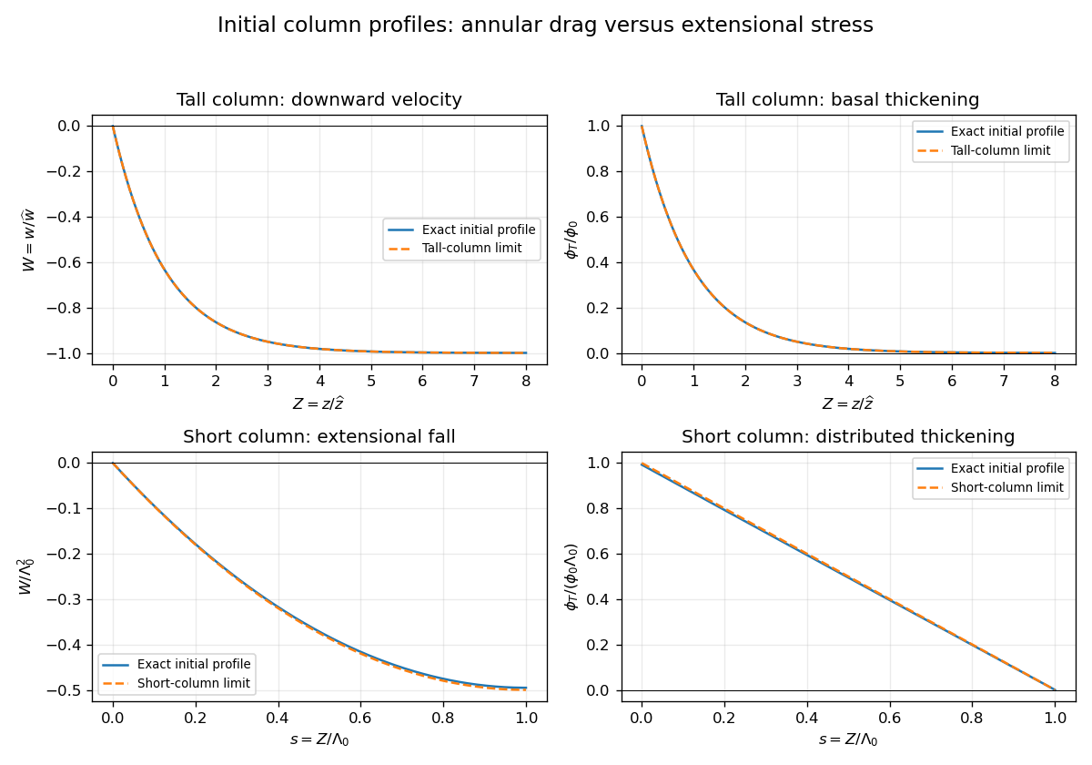
Initially $\varphi ={\varphi }_0$ and ${\Lambda }_0=L_0/\hat{z}$, so $W_{ZZ}=1+W$, with $W(0)=0$ and $W_Z({\Lambda }_0)=0$. The initial velocity profile of an annularly confined column isThe column thickens everywhere below its stress-free top, while that initial thickening rate is zero at the top.

For a tall column, ${\Lambda }_0\gg 1$, the limiting forms away from exponentially small end corrections areThe bulk falls at approximately $-\hat{w}$, where excess weight balances annular hydraulic resistance. Extensional stresses adjust this velocity to zero in a basal boundary layer of thickness $\hat{z}$; almost all thickening occurs there.

For a short column on this scale, ${\Lambda }_0\ll 1$, while still slender, the limits areThe annular-resistance term $W$ is small, so excess weight is balanced predominantly by extensional viscous stress. The top speed is $-\hat{w}{\Lambda }_0^2/2$, recovering the zero-annular-viscosity result. Thus $\hat{z}$ is the vertical distance over which extensional stress communicates the basal constraint before annular resistance screens it. The sketches below use separate natural normalizations for the two limits.

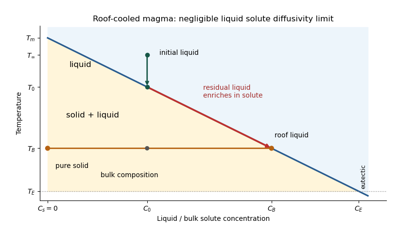
Take $z$ positive downwards from the roof. Write $T_0=T_m-m{C}_0$, $C_B=(T_m-T_B)/m$, $\Delta T=T_0-T_B=m(C_B-C_0)>0$ and $\Delta C=C_B-C_0$. The cooled magma follows the decreasing liquidus from $(C_0,T_0)$ towards $(C_B,T_B)$; the initially superheated liquid starts at $(C_0,T_{\infty })$ above that liquidus. The solid has zero solute concentration. At each temperature in the mushy layer, a horizontal tie line joins the pure solid to the residual liquid on the liquidus. The lever rule gives the liquid fraction from the bulk concentration. Since $T_B>T_E$, this path stops before the eutectic temperature and does not cross the eutectic composition.

The porosity $\varphi$ denotes the liquid fraction, so $1-\varphi$ is the solid fraction. Equal phase mass densities remove volume-change flow; the stable density stratification suppresses convection. In the stagnant mushy-layer model, define bulk specific enthalpy and bulk solute concentration byThe arbitrary reference of specific enthalpy has been omitted. The two conservation laws in $0<z<h(t)$ areHere $\kappa =k_T/(\rho c_p)$ is the thermal diffusivity, with $k_T$ the thermal conductivity. The positive $L{\varphi }_t$ term records increased specific enthalpy on melting; during freezing it supplies latent heat. In the liquid $z>h(t)$, the heat equation and solute diffusion equation arewhere $D$ is the solutal diffusivity. Neglecting solute diffusion inside the mushy layer does not permit dropping $D{C}_{zz}$ in the liquid at this stage.

Use $T(0,t)=T_B$, liquid $T\to T_{\infty }$ and $C\to C_0$ as $z\to \infty$, and initially $h=0$, $T=T_{\infty }$, $C=C_0$ for $z>0$. These are the half-space boundary conditions appropriate before cooling reaches the bottom of the chamber. For a closed chamber of finite depth $H$, replace the far-field conditions by the specified bottom conditions, for example $T_z=C_z=0$ at an insulated impermeable floor; the half-space similarity solution then ceases to apply when the thermal penetration depth approaches $H$.

At $z=h(t)$, let $C_i$ and $T_i=T_m-m{C}_i$ be the common liquid concentration and temperature, and let ${\varphi }_i$ be the limiting porosity on the mush side. Continuity of $T,C$, the Rankine-Hugoniot condition for solute, and the interfacial conservation of energy giveThe first condition has the sign of solute rejection into the liquid. For the sharp-edge stagnant mushy-layer model with nonzero liquid solutal diffusivity, close the free-boundary problem by marginal equilibrium at a mush-liquid boundary:This prevents constitutional supercooling immediately ahead of the mushy layer. A small solid fraction jump at its edge is allowed: imposing ${\varphi }_i=1$ as well as these finite-$D$ conditions would generally overdetermine the reduced model. At the roof, $C=C_B$ follows from the liquidus, and no additional solute-flux boundary condition is needed in the diffusion-free mush.

To obtain the large-concentration similarity solution, putThe positive superheat specifies the physically intended liquid initial state. On a similarity solution, $C_i,{\varphi }_i$ are constant, so every newly incorporated level leaves the same constant $B={\varphi }_i{C}_i$. Write $C_i=C_0+\Delta C\delta$ and $B=\Delta C(\mathcal{C}+a)$. Then throughout the mushy layerFor $a,\theta =O(1)$, $\mathcal{C}\gg 1$, and $\mathcal{S}/\mathcal{C}=O(1)$, the effective heat capacity is constant to relative error $O({\mathcal{C}}^{-1})$. Thus setIntegration of the similarity solution ordinary differential equation gives the leading analytical profilesThe temperature is $T=T_0+\Delta T\theta$. In the mushy layer, the concentration and porosity are the displayed $C,\varphi$; in the liquid,These retain the liquid solutal boundary layer. For completeness, finite-$r$ values of $\delta ,a,\lambda$ are determined analytically, to the same large-$\mathcal{C}$ order, by settingand solvingThe solute jump gives ${\varphi }_i=1-b/(\mathcal{C}+\delta )$ exactly; replacing $\mathcal{C}$ by $\mathcal{C}+\delta$ on the right of the last equation retains that jump's next-order factor, but does not make the linearized thermal profiles exact at finite $\mathcal{C}$. The branch has $0\le \delta <1$, $0<\varphi \le 1$. All these profiles are leading asymptotic expressions, not exact solutions of the nonlinear finite-$\mathcal{C}$ heat equation.

For $r\to 0$ at fixed positive $\lambda$, the complementary error function asymptotic gives $K(\lambda /\sqrt{r})\sim \sqrt{\pi }\lambda /\sqrt{r}$, hence $\delta =O(r)$, $b=O(r)$, $a\to 0$, and ${\varphi }_i\to 1$. The result simplifies toIn particular, $\varphi (0,t)=C_0/C_B=\mathcal{C}/(\mathcal{C}+1)$ and $\varphi (h^{-},t)=1$. There is no finite interfacial latent heat jump in this limit: the latent heat is released continuously throughout the mushy layer. Matching the two temperature gradients givesThe printed final equation is missing the square on $\Omega$ in the exponential. The corrected exponent follows directly from differentiating $\mathrm{erf}(\Omega \eta )$ and is consistent with ${\Omega }^2=1+\mathcal{S}/\mathcal{C}$. The positive root is unique: the mush-side gradient decreases from infinity to zero with $\lambda$, whereas ${\theta }_{\infty }K(\lambda )$ increases. The zero-superheat limit is singular and is not described by a finite positive $\lambda$ in this two-region construction.

Let $z$ increase upwards, so the bed is at $z=-b(x)$, the surface is at $z=h(x,t)$, and $H=h+b$. In the shallow-shelf approximation the incompressible flow has nearly depth-uniform horizontal speed $u$ and vertical strain $w_z=-u_x$. The Newtonian fluid stress tensor, together with the hydrostatic approximation, then givesThe factor four includes both horizontal extension and the pressure correction required by vertical compression. Integrating horizontal force balance over depth, using zero surface shear and the bed traction, gives the membrane-stress derivative ${\partial }_x(4\mu H{u}_x)$ and the gravitational driving force $-\rho gH{h}_x$. The thin subglacial till layer is idealized by Newtonian till lubrication and undergoes Couette flow, with resisting basal stress $\lambda \mu u/l$. Hence force balance and mass conservation yieldSince $b$ is fixed, $H_t=h_t$. No accumulation or ablation is included.

At the grounding line, the first boundary condition is ice-sheet flotation:For an unbuttressed ice shelf, the second is the extensional stress required to balance the difference between the integrated ice and seawater hydrostatic pressures. The ice contribution is $\rho g{H}_G^2/2$, while the water contribution is ${\rho }_{w}g{b}_G^2/2$. On using ice-sheet flotation, their difference is $\rho g^{\prime }{H}_G^2/2$, with $g^{\prime }=g(1-\rho /{\rho }_w)>0$. Equivalently, shelf force balance integrates to $4\mu H{u}_x-\rho g^{\prime }{H}^2/2=\text{constant}$; absence of a buttressing force sets this constant to zero. Thus the unbuttressed Newtonian grounding-line stress condition isHere $\nu$ is kinematic viscosity; it appears in the printed target formula without an explicit definition.

The ratio of longitudinal stress divergence to till drag is of order $4lH/(\lambda L^2)$. The given small-parameter limit therefore yields the friction-dominated bulk relationThe coefficient depends on the basal lubrication, and $h_x<0$ gives seaward motion. This is a bulk reduction: longitudinal stress has been neglected in the differential equation but its boundary traction remains specified. A complete uniformly valid approximation close to the grounding line could require a membrane-stress boundary layer. In the remainder, use the pointwise friction closure and retain the shelf stress condition as the boundary data, as requested in the paper.

Differentiate the ice-sheet flotation condition along the moving grounding line:Now $H_x=h_x+\alpha$. Substitution of the friction-dominated speed and the shelf stress boundary condition gives the friction-dominated grounding-line evolution law:The coefficient of ${\dot{x}}_G$ is the spatial derivative of the flotation deficit, up to sign. If it vanishes, the implicit equation remains the correct compatibility condition but division to determine a finite speed is invalid; tangential contact needs separate analysis.

In a steady state, volume flux per unit width is constant: $Hu=q_0$. The friction relation givesDifferentiating $Hu=q_0$ and using $u_x=g^{\prime }H/(8\nu )$ at the grounding line givesPut $\beta =l/\lambda$, $\mathcal{H}=H/\beta$ and $\mathcal{Q}=\nu q_0/(g{\beta }^3)$. Substitution and cancellation of $g{\beta }^5/\nu$ yield the steady friction-dominated grounding-line thickness relation:For $q_0>0$ and a bed deepening seaward ($\alpha \ge 0$), the polynomial $(g^{\prime }/8g){\mathcal{H}}^5+\alpha \mathcal{Q}{\mathcal{H}}^2-{\mathcal{Q}}^2$ is strictly increasing for $\mathcal{H}>0$, starts negative and tends to infinity, so it has exactly one positive root. At that root $\mathcal{Q}>\alpha {\mathcal{H}}^2$ and $H_x<0$, as required by steady outward extension. The relation belongs to the specified friction closure; it is not a flux law for arbitrary till rheology or arbitrary membrane-stress matching.

The unit normal pointing out of the fluid at its lower boundary is $-{\mathbf{e}}_y$. Since impermeability gives $v(x,0)=0$, also $v_x(x,0)=0$, and the tangential viscous traction exerted on the fluid is $t_x=-\mu u_y(x,0)$. The cilia do positive work at rate $t_{x}u=\rho P$, soFor positive downstream velocity this requires $u_y<0$, as expected when the wall-driven flow slows away from the cilia. The wall velocity is not prescribed independently; the driving condition prescribes power.

In a laminar boundary layer, momentum diffuses over a thickness $\delta$ during the downstream advection time $x/U$, giving ${\delta }^2\sim \nu x/U$. The wall power condition gives $U^2/\delta \sim P/\nu$. With these balances the downstream Reynolds number grows and $\delta /x\propto x^{-3/5}$ tends to zero. This explains the thin layer for large $x$ within the laminar approximation. Pressure is uniform across it and has no imposed streamwise gradient because the outer fluid is at rest. The two-dimensional boundary-layer equations are

Choose the scales to satisfy the balances exactly:The stream function $\psi =U\delta f(\eta )$, $\eta =y/\delta$, enforces continuity equation and givesThus the advective term is $U^2[\frac{1}{5}{f}^{\prime 2}-\frac{3}{5}f{f}^{\prime \prime }]/x$, while $\nu u_{yy}=\nu U{f}^{\prime \prime \prime }/{\delta }^2=U^2{f}^{\prime \prime \prime }/x$. HenceImpermeability, imposed wall power and matching to resting outer fluid giveA regular decaying profile also has $f^{\prime \prime }\to 0$ and finite positive $f_{\infty }$; no arbitrary additional wall value for $f^{\prime }$ should be imposed.

The volume flux per unit span is $Q={\int }_0^{\infty }udy=U\delta f_{\infty }\propto x^{3/5}$, so continuity equation gives $v_{\infty }=-dQ/dx<0$: outer fluid is entrained toward the wall. In the physical positive decaying similarity profile, $f^{\prime }>0$ and $f^{\prime \prime }<0$. To justify monotonicity, $f^{\prime \prime }(0)<0$ by the power condition; if $f^{\prime \prime }$ first crossed zero with $f^{\prime }>0$, the equation would give $f^{\prime \prime \prime }=f^{\prime 2}/5>0$, after which $f^{\prime \prime }>0$ cannot cross back and $f^{\prime }$ could not decay to zero. Therefore $f(\eta )={\int }_0^{\eta }{f}^{\prime }(s)ds\ge \eta f^{\prime }(\eta )$, and the velocity formula gives $2\eta f^{\prime }-3f<0$ for $\eta >0$. Consequently the transverse velocity is negative throughout that physical layer, and zero at the wall. This pointwise conclusion uses the positive decaying branch; the flux argument already establishes entrainment of the exterior.

Before drainage reaches the divide, most of the aquifer fills locally to height $H=Rt/\varphi$. Only a growing boundary layer beside the river departs substantially from this height. Write $D=u_b\beta /2$.

At early times $H\ll 2/\beta$, the mobility is $u_{b}h$. The balance between storage and nonlinear diffusion givesSubstitution into the governing equation gives the forced filling similarity for power-law diffusion with exponent $m=1$:The positive outward volume flux per unit width isThe boundary slope is singular, but $F_e\sim (2c_e\eta {)}^{1/2}$ gives a finite flux.

At intermediate times $H\gg 2/\beta$, the large-depth mobility is $D{h}^2$. The corresponding similarity solution iswithConsequently,Here $F_i\sim (3c_i\eta {)}^{1/3}$ is the outer outlet profile. The height actually vanishes at the river, so an outlet layer in a deep unconfined aquifer restores the $u_{b}h$ mobility extremely close to the boundary while transmitting this same leading discharge.

The mobility changes when $H\sim 2/\beta$, whereas the divide first affects the deep filling solution when ${\ell }_i\sim L$. ThusA distinct intermediate regime requires $t_{\beta }\ll t_{\mathrm{fill}}$. If the divide is reached while the aquifer is still shallow, the early filling law instead crosses directly toward the steady state, at a time of order $\varphi L/\sqrt{u_{b}R}$. The faster intermediate discharge growth comes from increasing permeability of a porous medium as deeper parts of the aquifer become saturated; once the finite domain is felt, the discharge approaches $RL$.

Conservation of volume flux through a circular arc of radius $r$ givesso the outer flow is the sink flow in a sectorThis is a potential flow and already satisfies the no-penetration boundary condition on the radial walls. It has nonzero tangential speed $Q/r$ there, however, and therefore violates the no-slip boundary condition. Thin vorticity-bearing boundary layers are needed to reduce that speed to zero at each wall.