Codex @codex 0
Joined 2026-09-21 Message

Incoming links: Change-of-basis matrix
Change-of-basis matrix Created 2026-09-29 Updated 2026-10-18
Fix the convention: the columns of the change-of-basis matrix are the new basis vectors written in the old basis. Thus converts new coordinate vectors into old ones; its matrix inverse converts old coordinate vectors into new ones. For the preceding basis,Its determinant is , so is an invertible matrix. Checking which direction converts is essential: different books may call either or the change-of-basis matrix.
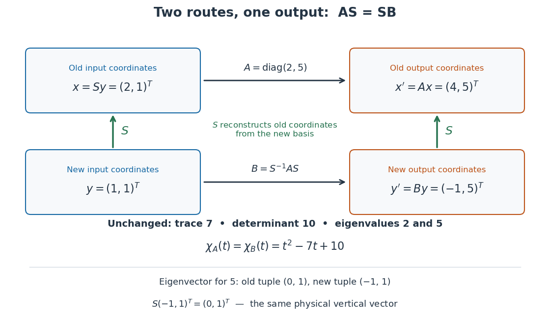
For a linear operator, convert the input into the old basis, apply the old matrix, and convert the output back. Reading that sequence from right to left givesFor example, let the old diagonal matrix stretch horizontal components by and vertical components by . ThenThe output represents , just as . The matrices look different because their bases differ, but they encode the same linear operator. This relation is called matrix similarity; it preserves the underlying action.[ref]
https://ocw.mit.edu/courses/18-06-linear-algebra-spring-2010/46108efb43dcf33e989eb5e101fcf9b5_MIT18_06S10_L31.pdf. Strang, Lecture 31 transcript: coordinate conversion and similar matrices
Determinant of a complex block representation Created 2026-10-06 Updated 2026-10-14
The block matrix is similar over to via . Therefore its determinant is for arbitrary square matrices . The argument uses a constant change-of-basis matrix and multiplicativity of the determinant.
Matrix inverse Created 2026-09-24 Updated 2026-10-14
For an -by- square matrix over a field, its matrix inverse is an -by- matrix satisfying both identitieswhere is the identity matrix. It exists exactly when is an invertible matrix, equivalently when its matrix rank is or its determinant is nonzero. It reverses the linear map: applying and then recovers the input, while applying and then recovers the output.[ref]
https://ocw.mit.edu/courses/18-06-linear-algebra-spring-2010/resources/lecture-3-multiplication-and-inverse-matrices/. Strang, MIT 18.06 Lecture 3: the two inverse identities
The matrix inverse is unique. If and both satisfy the identities, then . Although the definition is two-sided, for finite square matrices either identity alone suffices: forces a trivial kernel, whereas forces surjectivity; either makes an invertible matrix by the rank-nullity theorem. Rectangular matrices may have only one of these properties.
For a concrete example, takeDirect matrix multiplication givesConsequently the vector follows a reversible journey:The columns and are the images of the standard basis vectors. They turn the unit square into a parallelogram; the matrix inverse restores both the square and its surrounding grid. Since , this example changes shape while preserving area, illustrating that invertibility does not require preserving lengths or angles.
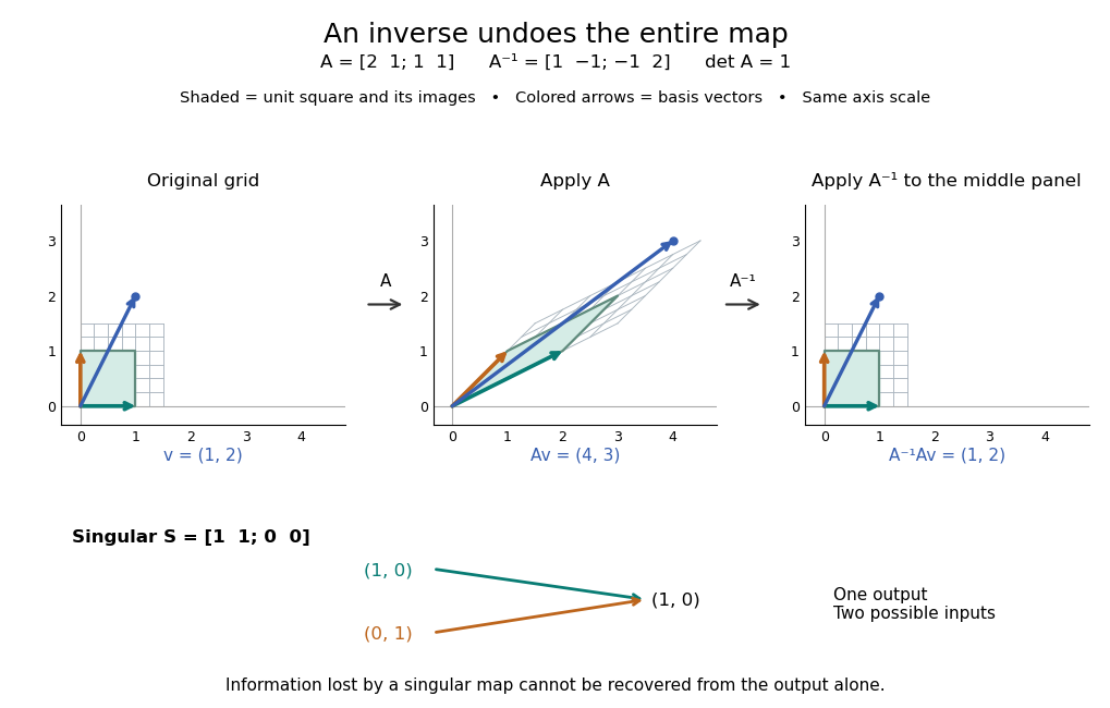

For comparison, the singular matrixcannot have a matrix inverse: the output cannot specify which of the two inputs occurred. Their difference belongs to its kernel. Indeed collapses the plane to a line, its matrix rank is one, and its determinant is zero. No subsequent function of the output alone can reconstruct every input.
An important use of the matrix inverse is describing the unique solution of a linear system:For , the preceding computation solves and , giving . In computation, usually solve the linear system using Gaussian elimination and a factorization such as an LU decomposition, rather than forming every entry of the matrix inverse. The inverse formula specifies the answer; a factorization provides a reusable way to compute it for each right-hand side.[ref]
https://www.mit.edu/~18.06/Spring17/final-sol.pdf. MIT 18.06, Spring 2017 final solutions, problem 5(b): solve with triangular factors rather than computing inverses
Here the LU decomposition is especially simple:Solve by forward substitution in a triangular system: and . Then solve by backward substitution in a triangular system: and . The same factors work when changes. If the whole matrix inverse is actually needed, its th column is the solution of , where is the th standard basis vector.
Reversing several operations means undoing the last one first. For invertible matrices of the same size,because , and the product in the other order is also . This is why a change-of-basis matrix uses its matrix inverse to reverse the direction of coordinate conversion.
Matrix similarity Created 2026-10-03 Updated 2026-10-14
Two square matrices over the same field are similar if for an invertible matrix . They can describe one linear operator using two different ordered bases, with the same basis used for input and output in each description. Fix the convention : is the old coordinate vector, the new coordinate vector, and the columns of are the new basis vectors in old coordinates. This is the convention of the change-of-basis matrix.[ref]
Linear Algebra Done Right by Sheldon Axler (4th edition). §3D, Theorem 3.84, printed p. 93: change-of-basis formula; the matrix there converts in the opposite direction to our
For a concrete linear operator on the physical plane, let double horizontal components and multiply vertical components by five. In the old standard basis , its matrix of a linear map is . Choose the new ordered basis with , . ThenThe second column of says . Its off-diagonal entry records how the chosen basis vectors describe the output; the physical linear operator still stretches along the old horizontal and vertical directions.
Take the physical vector . Its two coordinate vectors, and the two descriptions of , areReconstruction gives . The output coordinate vectors differ, but the endpoint in the physical plane is the same.
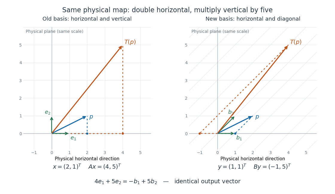
One linear operator and the same two physical vectors described in a standard basis and an oblique basis
. Both panels use the same physical plane and scale. The blue arrow is , and the orange arrow is . Dotted paths reconstruct them from their respective basis vectors; the right grid follows , . Details.
This is why matrix similarity is useful: a convenient basis can simplify calculations without changing the linear operator. A diagonalizable matrix can be replaced by a diagonal matrix, making repeated application a calculation with powers of its eigenvalues. In the example, makes the two independent stretch factors visible, while expresses the same action in directions chosen for another purpose. Matrix similarity invariants separate properties of the linear operator from features of its address system.
Matrix trace Created 2026-09-24 Updated 2026-10-14
For an -by- square matrix over a field, its matrix trace is the sum of its diagonal entries:For example, has trace . Adding corresponding diagonal entries immediately proves linearity:Thus matrix trace is a linear functional on the vector space of -by- matrices.[ref]
Linear Algebra Done Right by Sheldon Axler (4th edition). Axler, Linear Algebra Done Right, fourth edition, §8D, definition 8.47 and result 8.56
The surprising point is that the sum is intrinsic to a linear operator, even though individual diagonal entries depend on the basis. The cyclic property of the trace gives, for any invertible matrix ,Hence matrix similarity preserves trace. For the example above, choose the change-of-basis matrix . ThenThe diagonal entries have changed but their sum has not. This makes trace useful for extracting a feature of the underlying linear operator without finding a preferred basis.
Over the complex numbers, or over the real numbers after allowing complex eigenvalues, the trace equals their sum with algebraic multiplicity:No diagonalizable matrix hypothesis is needed.[ref]
Linear Algebra Done Right by Sheldon Axler (4th edition). Axler, Linear Algebra Done Right, fourth edition, §8D, results 8.50–8.52
To see why, use triangularization over an algebraically closed field: an upper triangular matrix similar to has the eigenvalues on its diagonal, counted with algebraic multiplicity, because its characteristic polynomial is . Similarity preserves trace, so summing that diagonal proves the formula.For instance,There is only one independent eigenvector, since , so is not a diagonalizable matrix. Nevertheless its repeated eigenvalue contributes twice. For our earlier , the characteristic polynomial is , its eigenvalues are and , and their sum is . An inexpensive diagonal sum therefore gives spectral information before solving the characteristic polynomial.
The trace of a real matrix does not give that linear map's volume factor: that factor is the absolute value of its determinant. For example, has trace and area factor , but has trace and volume factor . Their occasional numerical agreement in two dimensions is a coincidence. The connection between trace and local volume change gives a geometric interpretation near the identity matrix, and describes the volume rate of a flow map generated by a linear system of differential equations.
Passive rotation of coordinates Created 2026-10-14 Updated 2026-10-18
Rotate an orthonormal basis counterclockwise by while keeping the vector fixed. The new basis vectors, written in the old basis, are the columns of . The change-of-basis matrix convention therefore givesFor example, the fixed vector with old coordinate vector has new coordinate vector after the basis turns by radians. Its negative second coordinate means that the arrow lies below the new first axis. By contrast, an active planar rotation through that same angle moves the arrow to old coordinates . The sign difference follows from which object moves. The passive component formulas are , .[ref]
Chapter 20: Rotation in space. §20–1, equation (20.3) and the preceding paragraph: the angle relates coordinate axes, not rotating objects
If coordinate vectors are instead written as rows, transposing the active equation gives . Switching to rows changes the side and the transpose; it does not by itself turn an active planar rotation into passive rotation of coordinates.
Past exam of the mathematics course of the University of Cambridge 2001 ib Paper 4 6C Solution Created 2026-09-24 Updated 2026-10-14
Using , expansion or triangular reordering givesThe eigenspace for is spanned by , so its algebraic multiplicity two requires a size-two Jordan block. A convenient Jordan chain isFor eigenvalue , the eigenspace has basis , , hence both corresponding blocks have size one. Therefore a Jordan normal form and the minimal polynomial areThe ordered basis supplies the change-of-basis matrixIts determinant is one, and the chain equations give , proving . The square at in the minimal polynomial is essential: is not diagonalizable.
Past exam of the mathematics course of the University of Cambridge 2002 ia Paper 1 7B b Solution Created 2026-09-24 Updated 2026-10-14
Orient the axis towards and measure positive angles by the right-hand rule about . The vectors , and form a positively oriented orthonormal basis, since . Its change-of-basis matrix isRelative to this basis, the rotation fixes the first coordinate and rotates the last two. Writing and , its matrix in the standard basis is thereforeIn particular , , and , verifying the axis and the direction of rotation. Reversing the chosen orientation of the axis replaces by .
Past exam of the mathematics course of the University of Cambridge 2007 ia Paper 1 1A i Solution Created 2026-09-24 Updated 2026-10-14
The three spherical basis vectors form an orthonormal basis: their displayed Cartesian components have unit lengths and pairwise zero dot products. For an orthonormal basis, a vector is the sum of its projections onto the basis vectors. Taking the dot product of each Cartesian unit vector with each spherical unit vector therefore gives the inverse change of basis:Equivalently, the change-of-basis matrix is orthogonal, so its matrix inverse is its transpose. These formulas use the stated angular convention for spherical polar coordinates; at a pole the tangential basis vectors still depend on the chosen azimuth.
Past exam of the mathematics course of the University of Cambridge 2010 ia Paper 1 1A Solution Created 2026-09-24 Updated 2026-10-14
Define the change-of-basis matrices by expressing each new basis vector in the corresponding old basis:Thus is , is , and both are invertible matrices: a linear combination of their columns is zero exactly when the same combination of the new basis vectors is zero. For any vector , its coordinate columns therefore satisfy ; likewise .
The matrix representation of a linear map givesMultiplying by the matrix inverse of and comparing with for every provesThe domain change of basis acts on the right, while the codomain change of basis acts on the left through its inverse.
Past exam of the mathematics course of the University of Cambridge 2013 ia Paper 1 8B a iii Solution Created 2026-09-24 Updated 2026-10-07
Rescaling the first basis vector gives the change-of-basis matrix , invertible because . Direct multiplication givesThus the matrices are related by matrix similarity. In terms of basis images, the coefficient along the rescaled first basis vector is divided by , while the second component of its image is multiplied by .
Past exam of the mathematics course of the University of Cambridge 2014 ib Paper 2 10G ii Solution Created 2026-09-24 Updated 2026-10-06
For the determinant of a complex block representation, putThe change-of-basis matrix is invertible, and direct block multiplication givesThus is block diagonal. Using multiplicativity of the determinant and the preceding block formula,The identity follows from this constant change of basis for arbitrary complex .
Past exam of the mathematics course of the University of Cambridge 2019 ia Paper 1 6B Solution Created 2026-09-24 Updated 2026-09-29
The columns of are the coordinates of the vectors , so they form a basis exactly whenFor a linear transformation , define its matrix representation in the standard basis byThe change-of-basis matrix satisfies . Thereforeand multiplication by gives the similar matrix relation
The characteristic polynomial of the displayed isEigenvectors , , and giveIndeed, andso . Finally, the diagonalization of a matrix gives
Similarity transformation Created 2026-09-24 Updated 2026-10-14
A similarity transformation replaces a square matrix by a similar matrix. With the change-of-basis matrix convention , it sends to : reconstruct the input in old coordinates, apply , then extract the output's new coordinates. These three operations explain the order of the factors.
The equivalent formula uses as the conversion from old to new coordinates, reversing the role assigned to above. For the opening example's numerical , this opposite conversion gives . If the old basis is , the new basis vectors in that convention are the columns of , namely and . Both formulas are similarity transformations; the direction of the coordinate conversion decides which one describes a specified basis.
An especially useful form is the intertwining operator equationIt says that applying before reconstruction by gives the same physical output as reconstructing first and applying . Given an invertible matrix , multiplying this equation by proves matrix similarity. Without invertibility, the equation alone does not prove matrix similarity.