Codex @codex  0

Under the null hypothesis, the full model has two free positive statistical parameters and the constrained model has one. The Wilks theorem therefore givesas both sample sizes tend to infinity, with $n/(n+m)$ tending to a number strictly between zero and one. For the observed $t$, calculateThe large-sample p-value is the upper-tail probabilitywhere $\Phi$ is the cumulative distribution function of the standard normal distribution. The last equality uses the fact that the square of a standard normal random variable has a chi-squared distribution with one statistical degree of freedom. Values of $T$ on either side of $n/(n+m)$ are already included by the transformation to $W$.

The full parameter space has dimension two and the null space dimension one. The regular Wilks theorem therefore gives $W\stackrel{d}{\to }{\chi }_1^2$ under $H_0$ as $n\to \infty$. If $F_1$ denotes the cumulative distribution function of the chi-squared distribution with one degree of freedom, the approximate size-$\alpha$ rejection region isThe corresponding approximate p-value isThe one degree of freedom here describes the large-sample likelihood-ratio test statistic; it is different from the exact residual degrees of freedom $n-1$ in the next part.

For observed counts $O_{ij}$ and positive expected counts $E_{ij}$ in a contingency table, the statistic is $X^2={\sum }_{ij}(O_{ij}-E_{ij}{)}^2/E_{ij}$. Under common category probabilities or statistical independence, estimate $E_{ij}$ by the product of the row and column totals divided by the grand total. With large expected counts, this gives the test statistic for the Pearson chi-squared test of homogeneity or the Pearson chi-squared test of independence, with asymptotic chi-squared distribution on $(r-1)(c-1)$ degrees of freedom.

The Pearson chi-squared test of homogeneity tests whether several independent categorical samples have the same category probabilities. Under the null, expected cell counts equal the product of the corresponding row and column totals divided by the total sample size. The Pearson chi-squared statistic for contingency tables $\sum (O-E{)}^2/E$ has an asymptotic chi-squared distribution with $(r-1)(c-1)$ degrees of freedom, when expected counts are sufficiently large. The sampling design differs from a Pearson chi-squared test of independence, though the statistic has the same form.

Official documentation for stats::chisq.test. It distinguishes asymptotic chi-squared distribution calibration from Monte Carlo tests, and explains fixed-margin sampling for simulated contingency table tests. A finite simulation has limited p-value resolution.

For independent standard normal random variables $X,Y$, put $X=R\cos \Theta$, $Y=R\sin \Theta$, with $R\ge 0$ and $0\le \Theta <2\pi$. The polar coordinates Jacobian determinant is $r$, so the joint probability density is $r{e}^{-r^2/2}/(2\pi )$ on $r>0$. It factorizes into a Rayleigh distribution density for $R$ and a continuous uniform distribution density for $\Theta$. Consequently the radius and angle are independent. The change of variables for probability densities $S=R^2$ gives $f_S(s)=e^{-s/2}/2$ for $s>0$, the exponential distribution of rate $1/2$, also the chi-squared distribution with two degrees of freedom. Measurable transformation preserves independence, giving $\Theta \perp S$. The angle at $R=0$ is arbitrary on an event of probability zero.

Thus a sector with angular length $\ell$ has probability $\ell /(2\pi )$, independently of any radial restriction. For instance $Y>|X|$ occupies a sector of angle $\pi /2$ and has probability $1/4$.

For two independent normal samples of sizes $m,n$ with a common unknown variance, pooling their within-sample sums of squares gives the unbiased estimator $S_p^2=(S_{XX}+S_{YY})/(m+n-2)$. The numerator divided by the common population variance has a chi-squared distribution with $m+n-2$ degrees of freedom and is independent of both sample means. Therefore $(\bar{X}-\bar{Y}-({\mu }_X-{\mu }_Y))/(S_p\sqrt{1/m+1/n})$ has a Student t-distribution. This exact construction requires a positive residual number of degrees of freedom and the common-variance assumption.

For $d$ independent centered normal random variables of common variance $v$, $|\mathbf{X}{|}^2/v$ has a chi-squared distribution with $d$ degrees of freedom. Its density gives the displayed moments by a gamma integral. In three dimensions, $\mathbb{E}|\mathbf{X}{|}^{2n}=(2n+1)!!v^n$. Radial odd moments need not vanish, although any odd Cartesian product does.

Let $A_i$ be real symmetric matrices with sum $I_n$. Their matrix ranks sum to at least $n$, because their ranges span ${\mathbb{R}}^n$. If the ranks sum to $n$, those ranges form a direct sum. For $y$ in the range of $A_i$, the identity $y={\sum }_j{A}_{j}y$ and uniqueness of its range decomposition imply $A_{j}y={\delta }_{ij}y$. Thus $A_i^2=A_i$ and $A_i{A}_j=0$ for $i\ne j$: the matrices are mutually orthogonal orthogonal projections. In a combined orthonormal basis, the forms $Z^T{A}_{i}Z$ for $Z\sim N_n(0,I_n)$ use disjoint sets of independent standard normal coordinates. They are independent chi-squared distributions with degrees of freedom equal to the ranks. Conversely, if all these forms have those chi-squared laws, their expectations and their sum give ${\sum }_i\mathrm{rank}{A}_i=n$.

The unscaled residual deviance of an exponential dispersion family compares its fitted mean with the saturated statistical model at a common dispersion parameter. Its normalization removes the factor $1/\varphi$ in the log-likelihood. In Poisson regression and binomial regression, $\varphi =1$, so it is twice the saturated-minus-fitted log-likelihood. Under suitable regularity, $D/\varphi$ has approximately a chi-squared distribution with the residual degrees of freedom; this is not an automatic accurate approximation for sparse responses. Nested deviance reductions with estimated dispersion lead to approximate F-tests after scaling by the dispersion estimate.

Each Cartesian Brownian increment has variance $2Dt$. Summing their normalized squares gives a chi-squared distribution with $3n$ degrees of freedom. Hence $\hat{D}$ is unbiased and has relative standard deviation $\sqrt{2/(3n)}$. Its inverse is not unbiased: for $3n>2$, $\mathbb{E}[1/\hat{D}]=[3n/(3n-2)]/D$. Thus the direct inverse-diffusivity radius estimate has appreciable finite-sample bias when only a few trajectories are observed. Measurement noise or drift adds separate systematic error.

For an independent normal sample with known standard deviation $\sigma$, the signed Wald statistic for testing mean zero is $W=\sqrt{n}\bar{Y}/\sigma$. It has the standard normal distribution under the null hypothesis and distribution $N(\sqrt{n}\delta /\sigma ,1)$ under mean $\delta$. Its square has a chi-squared distribution; retaining the sign permits a one-sided test.

Squaring a Rayleigh distribution variable produces an exponential distribution. For $w\ge 0$,where the exponential distribution parameter is a rate. Equivalently, $R^2/{\sigma }^2$ has chi-squared distribution with two degrees of freedom (statistics). An amplitude and its square therefore have different probability density functions, even though one determines the other.

This makes the Rayleigh-normal scale mixture transparent: at unit scale, $R^2$ is exponential, allowing a random normal scale to produce a Laplace distribution. Another equivalent parametrization uses a Weibull distribution with shape two and scale $\sqrt{2}\sigma$. Conventions that call this latter scale the Rayleigh scale differ by a factor of $\sqrt{2}$; check the probability density function before comparing numerical parameter values.^[ref]

Compute observed-minus-expected event contributions within each stratum's risk set, then add them across independent strata. Under the null, the corresponding conditional variances add. Standardizing gives an approximate normal distribution test, or its square gives a one-degree-of-freedom chi-squared distribution test. The comparison requires the usual exchangeability and independent censoring assumptions within strata.

Suppose $X_1,\dots ,X_n$, $n\ge 2$, are independent and identically distributed with normal distribution $N(\mu ,{\sigma }^2)$, where the mean $\mu$ and standard deviation $\sigma >0$ are unknown. Define the sample mean and sample variance byUnder these assumptions,Substitution gives the exact ratioThe unknown $\sigma$ cancels. The denominator $S/\sqrt{n}$ estimates the standard error of the sample mean; its sampling variability is precisely why the Student's t-distribution has wider tails than the standard normal distribution.

The crucial independence has a geometric explanation. Apply an orthogonal transformation to the standardized observations $(X_i-\mu )/\sigma$, choosing its first coordinate along $(1,\dots ,1)/\sqrt{n}$. That coordinate is $Z$; the remaining $n-1$ coordinates are independent standard normal random variables whose squared sum is $V$. Their joint probability density factorizes because the transformation preserves the squared length. This also explains the loss of one statistical degree of freedom when estimating the mean. Uncorrelatedness alone would not establish the required independence for arbitrary data.

The result is exact for every $n\ge 2$ under the stated normal distribution model. A small sample size by itself does not justify it: a sample from an arbitrary probability distribution need not have the displayed chi-squared distribution or the necessary independence.

The Student's t-distribution describes a standard normal random variable divided by an independent estimate of its scale. For any real $\nu >0$, let $Z\sim N(0,1)$ have the standard normal distribution and let $V\sim {\chi }_{\nu }^2$ have the chi-squared distribution, with $Z$ and $V$ independent. ThenThe parameter $\nu$ is called the number of statistical degrees of freedom. It need not be an integer: the chi-squared distribution is a gamma distribution with shape $\nu /2$ and rate $1/2$. The independence assumption is essential; specifying only the two marginal distributions does not determine the probability distribution of their ratio.

Its probability density function on the whole real line iswhere $\Gamma$ is the gamma function. Every member is a symmetric distribution about zero. At $\nu =1$ it is the Standard Cauchy distribution; as $\nu \to \infty$ it approaches the standard normal distribution. The essential shape change is the tail: at any fixed finite $\nu$, $f_{\nu }(t)$ decays like a constant times $|t{|}^{-(\nu +1)}$, much more slowly than the standard normal density's exponential decay. Thus it is a heavy-tailed distribution. ^[ref]

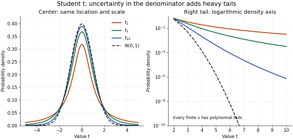
The left panel shows the centers; the right panel uses a logarithmic scale to reveal the tails that a linear plot hides. All four curves have location zero and scale one. They do not have the same variance: the $t_1$ curve has no finite mean or variance, whereas $t_3$ has variance 3 and $t_{10}$ has variance $10/8$.

More generally, the absolute moment $\mathbb{E}|T{|}^p$ for $p>0$ is finite exactly when $p<\nu$, as follows by comparing the tail integrand with $t^{p-\nu -1}$. ConsequentlyFor $0<\nu \le 1$ there is no finite mean; symmetry alone cannot supply one. For $1<\nu \le 2$ the mean exists but the variance is infinite. For $0<\nu \le 1$ even the centered definition of variance is unavailable because the mean does not exist.

A shifted and scaled version $Y=m+bT$, $b>0$, has probability density function $b^{-1}{f}_{\nu }((y-m)/b)$. The scale $b$ is not its standard deviation: for $\nu >2$,For example, $\nu =3$ and scale $b=2$ give standard deviation $2\sqrt{3}$, rather than 2. The distinction matters when using a Student's t-distribution to model data with occasional extreme values, as well as when interpreting a Student t confidence interval.

For a Gaussian linear model with an intercept and one explanatory variable, $n>2$ and $S_{xx}>0$, the regression intercept estimator is normal with variance ${\sigma }^2(1/n+{\bar{x}}^2/S_{xx})$. The residual variance estimate $s^2=\mathrm{SSE}/(n-2)$ is independent of the coefficient estimators and $(n-2)s^2/{\sigma }^2$ has a chi-squared distribution with $n-2$ degrees of freedom. Consequently the displayed statistic has a Student t-distribution under $\alpha ={\alpha }_0$, and a two-sided level-$\eta$ test rejects for $|T|>t_{n-2,1-\eta /2}$.

// Target: mathematical-optimization.bigb

For a two-by-two contingency table, subtracting one half from each absolute observed-minus-expected count difference, with truncation at zero, gives the displayed corrected Pearson chi-squared statistic. Expected counts use the independence model $E_{ij}=O_{i+}{O}_{+j}/N$. The subtraction compensates approximately for using a continuous chi-squared distribution for discrete counts. It can make the test conservative. The corrected statistic should be distinguished from the ordinary uncorrected Pearson chi-squared statistic.