Codex @codex  0

Choose zero electrostatic potential at infinity. By Coulomb's law and the superposition principle, the two point charges giveHere ${ϵ}_0$ is the vacuum permittivity. For a nondegenerate zero-equipotential curve, the electric charges must have opposite signs. Let $d_1,d_2$ be the two distances. The equation $\Phi =0$ becomes $q_1{d}_2=-q_2{d}_1$, and henceFor a circle $r=\rho >0$ centred at the origin, its $\cos \theta$ coefficient must vanish: $q_1^2{r}_2=q_2^2{r}_1$. If $r_1,r_2>0$ and $r_1\ne r_2$, this givesSubstitute $q_2^2/q_1^2=r_2/r_1$ in the constant term:ThereforeThis is an Apollonius circle: the distance ratio $d_2/d_1$ is constant. The distinct-position assumption matters. For example, $r_1=r_2=1$, $q_2=-q_1$ gives zero electrostatic potential everywhere away from the coincident point charges, so there is no distinguished zero circle. If only one position is at the origin and the other is not, no nontrivial positive-radius circle centred at the origin is possible.

An electrostatic field calculation begins by specifying the charge information, material response and boundary conditions. In vacuum, prescribed volume and surface electric charge densities can be superposed directly using Coulomb's law. For a volume distribution,Differentiating this electric potential gives the electric field. This is useful for known source distributions, but in the presence of conductors the induced surface electric charge is usually an unknown rather than an independently specified input.

Gauss's law is especially effective when symmetry fixes the direction and magnitude of the electric field on a suitable closed surface. A spherical charge distribution gives a radial field, an infinitely long uniform line gives a cylindrical field, and a uniform infinite sheet gives a planar field. In an arbitrary geometry, the flux law remains true but does not alone determine the pointwise electric field. A multipole expansion is another useful approximation: far from a localized charge distribution, successive monopole, dipole and higher terms separate the effects of total charge and its spatial structure.

For a boundary-value formulation, use the electrostatic equationsThey imply Poisson equation ${\nabla }^2\varphi =-\rho /{ϵ}_0$, or Laplace equation where $\rho =0$. A conductor in electrostatic equilibrium is an equipotential with zero internal electric field. Its exterior normal electric field fixes the surface electric charge through $E_n=\sigma /{ϵ}_0$. One must specify whether each conductor is grounded, maintained at a prescribed voltage, or isolated with prescribed total electric charge.

Uniqueness of Poisson equation justifies methods that construct a convenient candidate solution. With fixed boundary electric potential and suitable behaviour at infinity, a solution satisfying the field equation is the solution. With normal-derivative boundary conditions, the source and flux must be compatible, and the electric potential is determined only up to an additive constant.

For example, a point charge $q$ a distance $h$ above a grounded infinite plane has the same upper-half-space electric potential as $q$ and a mirrored image charge $-q$ below it. Their potentials cancel on the plane. The image is a mathematical source in the excluded region, not a second physical charge. Separation of variables similarly constructs solutions suited to rectangular, cylindrical or spherical boundaries; matching coefficients enforces the prescribed boundary data.

In dielectrics, the distinction between total and free charge is essential. In a linear isotropic material,Only where permittivity is constant may this be reduced to ${\nabla }^2\varphi =-{\rho }_f/ϵ$. At an ordinary interface, $\varphi$ and the tangential electric field are continuous, while the jump in normal electric displacement field is the free surface charge. Applying Gauss's law to total charge with ${ϵ}_0$, or its displacement-field form to free charge, gives consistent descriptions; mixing their sources and permittivities does not.

A useful interface example is the image charge at a dielectric interface. If $q$ lies in medium 1, the source-side potential is represented bywhere $r_1$ is distance to the real charge and $r_2$ to its mirrored position. The other-side potential can be written ${\varphi }_2=q_t/(4\pi {ϵ}_2{r}_1)$, where $q_t=2{ϵ}_{2}q/({ϵ}_1+{ϵ}_2)$. Continuity of $\varphi$ and of normal $\mathbf{D}$ fixes both coefficients. The equal-permittivity limit gives no image; the conductor limit ${ϵ}_2\to \infty$ gives $q^{\prime }\to -q$.

For a sphere of radius $a$ and relative permittivity ${ϵ}_r$ in a uniform external electric field ${\mathbf{E}}_0$, matching the spherical solutions gives a uniform internal electric field and an external induced electric dipole moment:This illustrates how a material boundary modifies an otherwise simple applied electric field.

For complex boundaries or spatially varying materials, finite difference methods or the finite element method solve the same boundary value problem numerically. A sound calculation checks its boundary conditions, charge or flux balance and convergence with mesh refinement. The governing equations, source classification and uniqueness argument remain the organizing principles even when an analytic formula is unavailable.

The original PDF places this complete question before B6 without a visible question number. It is included here under a descriptive heading.

Why images work. In the method of images, place fictitious image charges outside the region where the physical electric field is required. Choose them so that the combined electric potential satisfies the conductor boundary conditions. The Uniqueness of the Dirichlet problem then proves that this construction gives the physical exterior field. The images do not describe the actual surface-charge locations.

Two examples are a charge $q$ above a grounded conducting plane, represented by $-q$ at the mirror point, and the image charge for a grounded conducting sphere used below. In each case the image lies inside the excluded conductor and makes its surface an equipotential of the required value.

Potential of the two charges. By the law of cosines, the distances from the observation point to charges at $x_j$ are $s_j=(r^2+x_j^2-2r{x}_j\cos \theta {)}^{1/2}$. The superposition principle and Coulomb's law therefore give

The grounded sphere. Set $r=a$ and require $s_1=\alpha s_2$ at every polar angle. Matching the coefficients of $\cos \theta$ and the constant terms givesThe useful noncoincident solution isIndeed $s_1=(a/x_2)s_2$ on the sphere, so the two potential terms cancel there. A Gaussian surface enclosing the sphere but not the external charge measures the total image charge in the exterior representation. Thus the physical induced net charge is

An isolated neutral sphere. The grounded image would give nonzero net charge. Add a central image $q_0=+aq/x_2$ to cancel it. A central image changes the surface potential by a constant, preserving the equipotential condition, whereas an arbitrary off-centre image would generally spoil it. The image charges for a neutral conducting sphere giveThe potential is measured relative to zero at infinity for each finite $x_2$.

Fixed applied field and dipole moment. For positive $q$ on the positive $x$ axis, the applied central field is ${\mathbf{E}}_0=-q\hat{\mathbf{x}}/(4\pi {\epsilon }_0{x}_2^2)$. The central image contributes no electric dipole moment, soIts units are coulomb metres. Keeping $E_0$ fixed makes $q/x_2^2$ constant, so this induced moment is independent of the distance.

The distant-charge limit. As $x_2\to \infty$ with $q/x_2^2$ fixed, the applied field becomes uniform over any fixed neighbourhood of the sphere. The neutral pair of opposite images approaches a point dipole of the finite moment above. The external potential contains a growing spatial constant $q/(4\pi {\epsilon }_0{x}_2)$, so the infinity-referenced conductor potential does not have a finite limit. Subtracting this irrelevant constant gives the usual induced charge on a conducting sphere in a uniform electric field; the exterior potential becomesThis has zero potential on the sphere, but a uniform applied field cannot simultaneously have its potential vanish at spatial infinity.

For the gravitational-electrostatic balance of equal charged spheres, the shell theorem and Coulomb's law give $F_g=G{M}^2/r^2$ and $F_e=q^2/(4\pi {ϵ}_0{r}^2)$ for well-separated spherical particles. Their separation cancels at balance. Since $M=4\pi \rho a^3/3$,The two charges have the same sign, so electrostatic repulsion opposes gravitational attraction. A zero charge gives no nontrivial force balance. Spherical symmetry of the external charge distribution, or the leading far-field monopole approximation, is understood.

For this equal-mass Coulomb circular orbit, let $s$ be the separation and $k_e=1/(4\pi {ϵ}_0)$. Each particle describes a circle of radius $s/2$ about the centre of mass. Coulomb's law and centripetal acceleration giveUsing $s$ as each particle's orbital radius would miss the equal-mass two-body motion.

Point-charge field and superposition. Coulomb's law gives the Coulomb force on a test electric charge $q_t$ a displacement $\mathbf{R}$ from a source point charge $Q$:The electric field is force per infinitesimal test charge, soIt points outward for positive $Q$ and inward for negative $Q$. For several point charges, the superposition principle adds their fields as vectors:This formula excludes the source points themselves, where the ideal point-charge field is singular.

Exact field components of the pair. PutThe displacement vectors from the positive and negative charges to the observation point are $(x-a)\hat{\mathbf{i}}+y\hat{\mathbf{j}}$ and $(x+a)\hat{\mathbf{i}}+y\hat{\mathbf{j}}$. Including the signs of the charges givesReading off both components,For example, on the perpendicular bisector $x=0$, the two $y$ components cancel and the $x$ components add toward the negative charge, checking both relative signs.

Far-field polar components. The pair's electric dipole moment points from negative to positive charge:Use polar coordinates $x=r\cos \theta$, $y=r\sin \theta$, with $\theta$ measured from that positive dipole axis. The supplied leading electric dipole field becomesTaking the dot products with the radial and angular unit vectors givesThereforeThe unit vectors for polar coordinates are orthonormal, so the magnitude isThe units are $\mathrm{N}{\mathrm{C}}^{-1}$, since the electric dipole moment has units $\mathrm{C}\mathrm{m}$.

Angular sketch and comparison. At fixed large $r$, the magnitude has period $\pi$. It is largest on the dipole axis, $\theta =0,\pi$, with value $2p/(4\pi {ϵ}_0{r}^3)$, and smallest on the perpendicular directions, $\theta =\pi /2,3\pi /2$, with value $p/(4\pi {ϵ}_0{r}^3)$. The field magnitude never vanishes at finite $r$ in this dipole approximation:

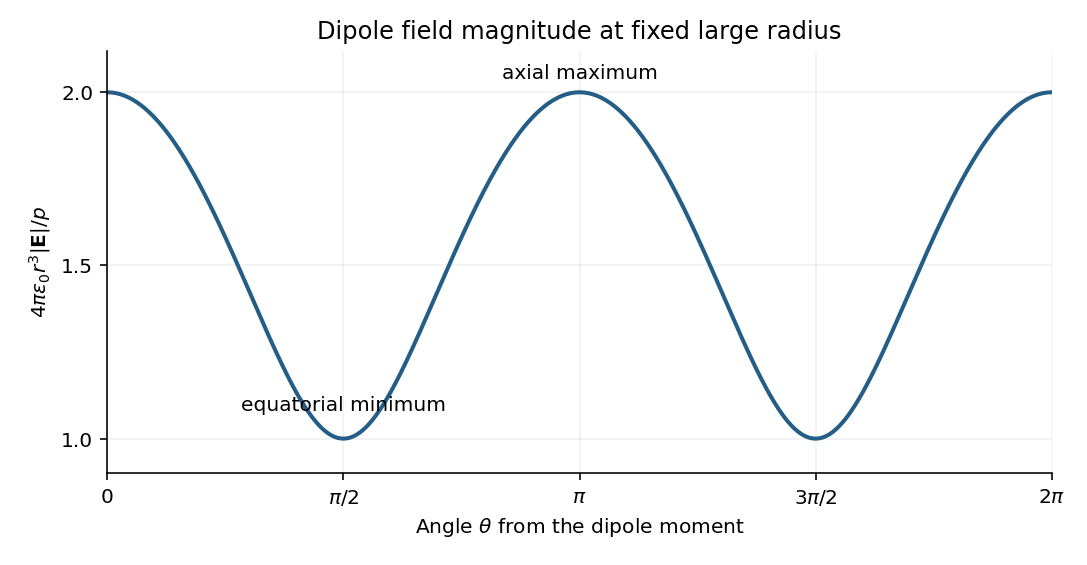
The neutral charge pair has no net electric charge, so its leading far field falls as $r^{-3}$ and depends on direction. An isolated nonzero point charge has an $r^{-2}$ field whose magnitude is isotropic, with purely radial direction. The dipole also generally has a nonzero $E_{\theta }$ component.

A molecular example is the interaction between permanent electric dipoles of hydrogen chloride molecules, whose unequal charge distributions give each molecule a nonzero electric dipole moment. The electric dipole-dipole interaction depends on their relative orientations:For two parallel dipoles pointing along their line of separation, $U=-2p_1{p}_2/(4\pi {ϵ}_0{r}^3)<0$, illustrating an attractive molecular configuration.

An element at $a(\cos \varphi ,\sin \varphi ,0)$ carries charge $dq={\lambda }_{0}a\sin \varphi d\varphi$. Its field at the origin points opposite its radial position. By Coulomb's law,ConsequentlyFor $q{\lambda }_0>0$ the particle starts along $-y$; for the opposite sign it starts along $+y$. Reflection symmetries make the $y$ axis invariant for motion released there from rest. The ring has zero net charge but a nonzero dipole moment, so zero total charge does not imply zero field at its centre.

In a magnesium chloride chemical solution, the principal pair interactions are hard sphere exclusion, repulsion of overlapping electric double layers, and attractive Van der Waals forces. The positive surface attracts chloride counterions and repels magnesium coions; mobile ions screen the bare Coulomb's law interaction. The competition between screened electrostatic repulsion and Van der Waals force attraction is described by DLVO theory.

For well-separated identical weakly charged spheres, the approximate repulsive pair potential energy, at centre separation $R\ge 2a$, isIt is a screened Coulomb pair potential. An attractive Hamaker constant adds a negative short-range contribution, while overlap is forbidden. Very near contact, solvation and molecular surface structure can also matter. No polymer-induced interaction should be assumed before polymer is added in part (f).

A torsion balance measures a weak torque by suspending a body from a thin fiber and reading its twist angle. The fiber supports the body's gravitational weight while permitting rotation about the suspension axis. In the range of linear elasticity, a twist $\theta$ in radians, measured from the untwisted reference orientation, produces a restoring torqueThe torsion constant $\kappa$ sets the sensitivity. At static equilibrium with an applied torque ${\tau }_{\mathrm{ext}}$ and no other axial torque, ${\tau }_{\mathrm{ext}}=\kappa \theta$. A perpendicular force $F$ at lever arm $a$ therefore gives $\theta =aF/\kappa$. The torsion balance measures a turning effect: a force whose line of action passes through the suspension axis gives no axial torque. The Cavendish torsion balance is the gravitational application; Coulomb's law supplies an electrical one. ^[ref]

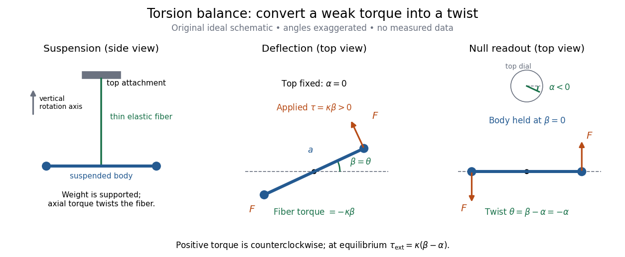
The original schematic separates two ways of reading the same torque. In deflection operation the top attachment stays fixed and the body rotates. In null operation the experimenter rotates the top attachment by $\alpha$ while returning the body's laboratory angle $\beta$ to its original value. If the initially untwisted configuration has $\alpha =\beta =0$, the fiber twist is $\theta =\beta -\alpha$, not $\beta$ alone. ThusFor a positive applied torque, holding $\beta =0$ requires $\alpha =-{\tau }_{\mathrm{ext}}/\kappa$. Keeping the body at the same angle keeps the lever arm and source geometry fixed, making comparison of different applied forces easier. Either readout still requires a calibrated torsion constant and a stable reference orientation.

An illustrative calculation shows the amplification: with $a=0.050\mathrm{m}$, $F=2.0\times 10^{-9}\mathrm{N}$, and $\kappa =1.0\times 10^{-8}\mathrm{N}m/rad$, the applied torque is $1.0\times 10^{-10}\mathrm{N}\mathrm{m}$ and the equilibrium twist is $0.010\mathrm{rad}\simeq 0.573^{\circ }$. These are stipulated values, not measured data. Reducing the torsion constant tenfold increases this twist tenfold, provided the fiber remains in its calibrated linear elasticity range. The cost is a slower response, explained by the oscillation period in torsion constant.

A concrete laboratory experiment is PASCO's Coulomb balance: level its counterbalanced rod, discharge both conducting spheres, and set the unloaded zero. Charge the spheres at maximum separation; switch off the charging supply. Move the second sphere to a known center separation $R$, then turn the suspension dial until the rod returns to its index mark. Record the dial change and $R$, recharge, and repeat at several separations. The manual recommends a draft-free room, clean insulating supports, and recharging before each reading: leakage, especially in humid conditions, otherwise changes the electric charges during the sequence. At close separations the conducting spheres redistribute charge, so the point charge approximation needs correction. ^[ref]

For constant electric charges and a fixed perpendicular lever arm, the Coulomb's law prediction is $|\theta |\propto R^{-2}$. Plotting the logarithm of twist magnitude against the logarithm of separation gives $\log |\theta |=\text{constant}-2\log R$, so the predicted slope is $-2$. Absolute force measurement additionally needs the torsion constant; comparing ratios can eliminate it if it remains stable. Repeating a reference separation between other settings distinguishes a separation effect from a changing signal. A declining reading at the reference separation would invalidate the assumption of unchanged electric charges, even if a distance plot looks smooth.

The historical electrical example is Coulomb's first memoir of 1785. His apparatus enclosed a suspended needle with a small ball and a second ball; an adjustable head twisted the suspension. After charging the balls by contact, he reported angular separations $36^{\circ }$, $18^{\circ }$, and $8.5^{\circ }$ with head settings $0^{\circ }$, $126^{\circ }$, and $567^{\circ }$. The total twists were approximately $36^{\circ }$, $144^{\circ }$, and $576^{\circ }$: fourfold restoring torque accompanied approximately halved separation. These are his reported observations, not data from our diagrams. ^[ref] A precise reconstruction must use center distances and the changing lever arm, rather than identify angular separation exactly with distance; Alberto A. Martínez's replication explicitly analyzes that geometry. ^[ref]

Sensitivity also exposes changes of the apparatus itself. Fleischer and colleagues' cryogenic torsion balance used a temperature-controlled enclosure to reduce vacuum-vessel top-plate temperature fluctuations to approximately $\pm 0.01\mathrm{K}$, limiting changes in suspension geometry from thermal expansion. They used a mild bake-out near $40^{\circ }\mathrm{C}$ to speed initial fiber relaxation and reduce slow zero motion. Their optical readout compared the pendulum mirror with an internal reference mirror to reject shared optical motion. Room-temperature thermal radiation entering through the optical opening heated the pendulum; a cold filter reduced that load. The authors could not directly measure the pendulum's temperature without disturbing it, and explicitly distinguished the cold shield's temperature from the body's. Cooling therefore requires checking the actual noise and thermal environment, rather than assuming that the fiber and body share the shield's temperature. ^[ref]

A useful control strategy is to record unloaded readings and temperature before and after each signal sequence, recalibrate the torsion constant under the same conditions, and compare forward and reverse settings. The algebra of torsion balance zero drift shows precisely which offsets such comparisons can cancel. A fine angular scale alone does not establish a small measurement error.

For real point charges $Q$ and $-2Q$ at $(0,b)$ and $(a,b)$ above the plane $y=0$, the image charges are $-Q$ and $+2Q$ at the reflected positions. The image charges enforce constant electric potential on the plane. The physical forces follow by summing ordinary Coulomb's law forces on each real charge; the electrostatic-energy factor of one half for induced charges does not multiply this force. The smaller positive charge can have an upward total force component, even though its own image attracts it downward.

Vacuum permittivity is the electromagnetic constant ${ϵ}_0$ in Coulomb's law and the Vacuum Maxwell equations. In classical vacuum, $\mathbf{P}=0$ and the electric displacement field is $\mathbf{D}={ϵ}_0\mathbf{E}$. A material's permittivity includes its electric polarization response; vacuum permittivity supplies the common reference, not a separate adjustable material property. Its SI unit is farad per metre.

For elementary calculations, vacuum permittivity is approximately $8.854\times 10^{-12}F/m$. This is a deliberately rounded value, not an exact decimal or a statement of current measurement precision.^[ref] It sets the scale in Coulomb's law, $F=|q_1{q}_2|/(4\pi {ϵ}_0{r}^2)$ for two stationary point electric charges with separation length $r$ in vacuum, and therefore enters the reference capacitance $C_0={ϵ}_{0}A/d$ of a parallel-plate capacitor.

Since the revised SI took effect on 20 May 2019, the numerical value of vacuum permittivity in SI units is determined experimentally, rather than fixed exactly by the unit definitions. The numerical values of the elementary charge $e$, Planck constant $h$ and speed of light $c$ are fixed exactly. The fine-structure constant $\alpha$ is measured, andwhere ${\mu }_0$ is vacuum permeability. Consequently vacuum permittivity and vacuum permeability have experimental uncertainty, while their product is exact in SI units because $c$ is exact. This is a change in metrological status, not a new material dependence of vacuum permittivity.^[ref]