Codex @codex  0

Integrating the probability density function from its lower endpoint to $x$ gives the cumulative distribution functionIt is continuous and strictly increasing on the support. Hence the unique median $m$ satisfies $F(m)=1/2$, or $m^{-\alpha }=1/2$. Therefore

Integrating the first probability density function gives the cumulative distribution functionIts graph is a straight ramp from $(0,0)$ to $(T_1,1)$, followed by a horizontal plateau.

The second cumulative distribution function is the integral of its density:Its graph is an upward-curving parabolic arc from $(0,0)$ to $(T_2,1)$, followed by a horizontal plateau. Both cumulative functions are continuous at their upper support endpoints.

The graph of the positive-delay probability density function is a horizontal segment at height $1/R$ from $s=0$ to $r$, followed by zero from $r$ to $R$. Values at individual endpoints do not affect probabilities. The separate atom $1-r/R$ at zero is not a finite-height part of this density graph.

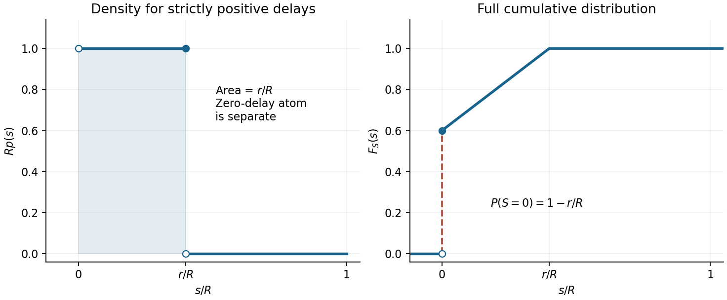
The companion cumulative distribution function in the figure is $F_S(s)=0$ for $s<0$, $F_S(s)=1-r/R+s/R$ for $0\le s<r$, and $F_S(s)=1$ for $s\ge r$. Its jump at zero displays the discrete part without confusing density height with probability mass.

For $s>0$, integrate the probability density function to obtain the cumulative distribution functionIf $\mu >0$, the requested probability is $F_X(\mu )-F_X(0)$. Since the hyperbolic tangent is odd, this givesThe second case matters because the question places no sign restriction on $\mu$: the event is empty when its upper endpoint is nonpositive. Using an oriented integral from $0$ to a negative $\mu$ would give a negative number, not a probability.

For a nonnegative integer $K$, add the probabilities of the disjoint events with $0,1,\dots ,K$ goals. The cumulative distribution function is

The angular interval has width $\pi$, so its continuous uniform distribution has probability density functionIntegrating this probability density function gives the cumulative distribution functionValues of the probability density function at the two individual endpoints may be assigned arbitrarily without changing any probability.

The tangent function is strictly increasing on the angular interval. Thus $Y\le y$ is equivalent, up to the zero-probability endpoints, to $\Theta \le \arctan (y/x_0)$. Substituting into the angular cumulative distribution function givesIts limits are zero and one at the two infinite endpoints. This is the construction in which the tangent of a uniform angle has a Cauchy distribution.

Differentiate the cumulative distribution function using the chain rule:This is a Cauchy distribution with location zero and scale $x_0$. The probability density function is nonnegative and integrates to $F(\infty )-F(-\infty )=1$.

Let $F$ be the cumulative distribution function of $X$. Normalisation of the proposed probability density function requires $M={\int }_{-2}^{2}F(y)dy$. The integrated cumulative distribution function on a bounded interval identity givesFor a direct symmetry proof, the continuous symmetric probability distribution satisfies $F(-y)=1-F(y)$. HenceIn particular $g(y)=F(y)/2$ is nonnegative and has total integral one over its stated support.

Because $X$ takes values only in $[0,1]$, its cumulative distribution function must satisfy $F(1)=1$. Thus

The full cumulative distribution function isThus the function graph is horizontal at zero for $-1\le x\le 0$, rises continuously from $(0,0)$ to $(1,1)$, and is horizontal at one for $1\le x\le 2$. Its derivative $12x^2(1-x)$ is positive on $(0,1)$ and zero at both endpoints. The second derivative $12x(2-3x)$ changes sign at $x=2/3$, giving an inflection point there.

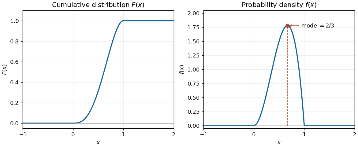
The probability density function is the derivative of the cumulative distribution function:It is nonnegative and has integral $F(1)-F(0)=1$. This is a beta distribution with parameters $3$ and $2$.

At the mode, the cumulative distribution function has valueSince $F$ is strictly increasing on $(0,1)$, its unique crossing of $1/2$ occurs earlier. Therefore the median is less than the mode.

The requested bounds are $\mathbb{E}[X]-\sigma =2/5$ and $\mathbb{E}[X]+\sigma =4/5$, both within the support. Since the probability distribution is continuous, endpoints have zero probability, and subtraction of the cumulative distribution function givesThis leaves the answer in rational fractions as requested.

Keep $a$ general initially, since the final part does not explicitly fix it. For $-h\le y\le h$, where $h=\pi /6$, the cumulative distribution function isThe normalization constant in the probability density function of $Y$ must beEquivalently, the integrated cumulative distribution function on a bounded interval identity gives $M=h-\mathbb{E}[X]$. If the assumption $a=0$ from part (c) is retained, the requested special case is $\boxed{M=\pi /6}$. For the value $a=1$ in part (b), it is $M=\pi /6-{\pi }^3/324$.

Write $d\mu =f(x)dx$, with $f\ge 0$. Applying polar coordinates and Fubini's theorem gives, for bounded nonnegative measurable $h$,Also $\tilde{\mu }(\{0\})=\mu (\{0\})=0$ by absolute continuity of measures. Extending $g$ by zero on the negative half-line proves

Both radial pushforward measures have compact support of a measure, so Brenier's theorem on the line supplies a unique optimal transport plan and a transport map $\tau$, unique $\tilde{\mu }$-almost everywhere, withIn one dimension, the gradient of a convex function is a nondecreasing function. Nonnegativity holds $\tilde{\mu }$-almost everywhere because ${\tau }_{\#}\tilde{\mu }=\tilde{\nu }$ is carried by $[0,\infty )$. To choose a nonnegative, nondecreasing representative everywhere, let $F,G$ be the radial cumulative distribution functions and use the monotone rearrangementAt $F(r)=0$ set $\tau (r)=0$, and at $F(r)=1$ use the largest point of the support of a measure $\tilde{\nu }$. These choices preserve monotonicity and boundedness. Since $F$ is continuous, $F(R)$ has the uniform distribution on $(0,1)$ when $R$ has law $\tilde{\mu }$, and the quantile function $G^{-1}$ sends this uniform distribution to $\tilde{\nu }$. Thus this representative has the required pushforward measure, even if the target has atoms.

By continuity of the cumulative distribution function and nonnegativity, $F(0)=0$; strict increase and $F(x)\to 1$ allow inversion for every $0<t<1$. The probability integral transform follows fromThus $F(X)$ is uniformly distributed on $(0,1)$.

The order statistics arrange the sample increasingly: $X_{(1)}\le \cdots \le X_{(n)}$. Strict monotonicity means $F(X_{(i)})$ is the $i$th order statistic of $n$ independent uniform variables. Its density isobtained by choosing the $i-1$ observations below $t$ and the $n-i$ above it. This is the beta distribution with parameters $i,n+1-i$, soFor the given log-logistic distribution, rearrangement givesConsequently plot $y_i=\log (i/(n+1-i))$ vertically against $x_i^{\ast }=\log X_{(i)}$ horizontally. Under a good fit, replacing $F(X_{(i)})$ by its plotting position $i/(n+1)$ gives an approximate straight line withThis is a diagnostic probability plot, rather than an assertion that the expectation of the nonlinear transformed order statistic equals that transformed plotting position. Positive observations occur almost surely under the model.

The central limit theorem states that for independent identically distributed variables of finite mean $\mu$ and positive finite variance ${\sigma }^2$,For a continuous strictly increasing cumulative distribution function, its inverse is defined on $(0,1)$. Thus $\mathbb{P}(F(X)\le y)=\mathbb{P}(X\le F^{-1}(y))=y$ for $0<y<1$, proving the uniform law.

If $T=-\log (1-Y)$, then for $t\ge 0$, $\mathbb{P}(T\le t)=\mathbb{P}(Y\le 1-e^{-t})=1-e^{-t}$. Hence $f_T(t)=e^{-t}{1}_{(0,\infty )}(t)$, an exponential density of rate one. Its first two moments are one and two, by integration by parts, so $\mathbb{E}T=1$ and $\mathrm{Var}T=1$.

Although the original variables may have different distributions, their separate transforms $Y_k=F_k(X_k)$ are independent and all uniform. Consequently $T_k=-\log (1-Y_k)$ are independent identically distributed exponentials of rate one, and the statistic is exactlyThe stated central limit theorem therefore yields $\boxed{Z_n\stackrel{d}{\to }N(0,1)}$.

For $x\ge 0$, the geometric distribution tail givesFor $x<0$, $P(T_k\le x)=0$. The limiting cumulative distribution function is therefore $0$ for negative $x$ and $1-e^{-x}$ for nonnegative $x$, and it is continuous everywhere. This proveswith rate parameter $1$ and mean $1$.