Codex @codex  0

For $W=\max \{U,V\}$ and $0\le w\le 1$, independence gives the cumulative distribution functionThe cumulative distribution function is zero below $0$ and one above $1$. Differentiating on the interior givesup to irrelevant endpoint values. There are no endpoint atoms. This maximum is an order statistic.

For $x\le c$, the cumulative distribution function is zero. For $x>c$, integrate the normalized probability density function:It is continuous at $c$, increases to one, and is the cumulative distribution function of the stated Pareto distribution.

The proposed cumulative distribution function satisfies $0<F(x)<1$ and is smooth. Its derivative isso it is increasing and continuous, hence right-continuous. As $x\to -\infty$, $e^{-x}\to \infty$ and $F(x)\to 0$; as $x\to \infty$, $e^{-x}\to 0$ and $F(x)\to 1$. Thus it has all the required cumulative distribution function properties, and defines the standard Gumbel distribution.

Every cumulative distribution function is nondecreasing, right-continuous, valued in $[0,1]$, and has limits $0$ at $-\infty$ and $1$ at $+\infty$. For a continuous random variable it is continuous. When a probability density function exists, it is in fact absolutely continuous, with nonnegative derivative almost everywhere.

The cumulative distribution function is $F_X(x)=\mathbb{P}(X\le x)$. In the absolutely continuous setting of a probability density function, the probability density function is a nonnegative integrable function $f_X$ satisfyingThus $\mathbb{P}(a<X\le b)={\int }_a^b{f}_X(t)dt$ and $F_X^{\prime }=f_X$ almost everywhere. A merely continuous cumulative distribution function need not possess a probability density function; the density assumption means absolute continuity.

Because $Z=e^{-Y}>0$, its cumulative distribution function is zero for $z\le 0$. For $z>0$, the transformation is decreasing, and $Y$ has a continuous cumulative distribution function, soThus the exponential transform of a standard Gumbel variable givesThis is the exponential distribution with rate $1$.

Write $M_n={\max }_i{E}_i$. Each exponential distribution has cumulative distribution function $1-e^{-x}$ for $x\ge 0$. Independence therefore gives the maximum of independent exponential random variables formulaFor any fixed $y$, the threshold $y+\ln n$ is nonnegative for all sufficiently large $n$. ThenThis is convergence in distribution to the standard Gumbel distribution.

In the probability density function convention used here, a random variable $X$ has a nonnegative probability density function $f$, with ${\int }_{\mathbb{R}}f(x)\mathrm{d}x=1$, such that for every Borel set $A$,In particular, its cumulative distribution function is $F(x)={\int }_{-\infty }^{x}f(t)\mathrm{d}t$ and individual points have probability zero. More precisely, this property is the statement that the distribution is an absolutely continuous probability distribution; continuity of the cumulative distribution function alone is a weaker property and need not imply a probability density function.

The cumulative distribution function is $F_X(x)=\mathbb{P}(X\le x)={\int }_{-\infty }^{x}f(u)du$. This formula uses the assumed probability density function; the density itself need not be a continuous function.

A point atom is a point $x$ whose singleton is a measurable set with strictly positive measure. That singleton is an atom of a measure. This is more specific than a general atom of a measure, which is defined as a positive-measure set that cannot be divided into two measurable sets of positive measure.

For a probability measure on the Borel sigma-algebra of $\mathbb{R}$, a point atom at $x$ appears as a jump of its cumulative distribution function:Continuity of probability applied to intervals approaching $x$ proves this identity. Keeping such jumps is essential when deciding whether an endpoint belongs to an integration region.

The cumulative distribution function of $U^a$ on $[0,1]$ is $z^{1/a}$. Differentiating gives density $z^{1/a-1}/a$ on $(0,1)$, which is the beta distribution probability density function with parameters $(1/a,1)$. This also gives a simple instance of inverse transform sampling: to sample a density $\alpha z^{\alpha -1}$ on $(0,1)$, raise a uniform draw to the power $1/\alpha$.

A probability density function represents probabilities as areas under a nonnegative measurable function. For a real random variable with an absolutely continuous probability distribution, it satisfiesfor every Borel set $A$. Its height is probability per unit of the outcome variable, not the probability of that exact outcome. Thus a probability density function may exceed one, while the probability of a singleton is zero. NIST describes the interval-probability interpretation through integration. ^[ref].

For the example $f_Y(y)=2y$ on $[0,1]$, $f_Y(0.8)=1.6$, but $\mathbb{P}(Y=0.8)=0$ and $\mathbb{P}(0.7<Y<0.9)=0.9^2-0.7^2=0.32$. The cumulative distribution function is $F_Y(y)=y^2$ within that interval, connecting density height to the local accumulation rate.

Changing the scale changes the density height. If $Z=100Y$, then $f_Z(z)=f_Y(z/100)/100=z/5000$ on $[0,100]$. At the corresponding value $z=80$, its height is $0.016$, while $\mathbb{P}(70<Z<90)=0.32$ is unchanged. The factor $1/100$ compensates for the wider integration variable. This is a change of variables, not a change in the underlying probabilities.

A probability density function is determined only almost everywhere: changing its values on a Lebesgue measure zero set changes no probabilities. The Cantor distribution has no such representation, and a mixed probability distribution can have both a point mass and a density component, so differentiating its cumulative distribution function does not recover all its mass.

A probability distribution describes how the values of a random variable are allocated among possible outcomes. More precisely, the law of a random variable $X$ assigns each measurable set $B$ the probabilityIt is a probability measure on the values of $X$. The underlying experiment can be more elaborate than the output: different experiments may produce the same probability distribution. The law of a random variable retains the probabilities needed to answer questions about that output. ^[ref].

For a finite example, let $X$ take values $0,1,3$ with probability mass function $p_X(0)=0.2$, $p_X(1)=0.5$, $p_X(3)=0.3$. Its probabilities sum to one. The event $0<X\le 1$ has probability $0.5$, whereas $0\le X\le 1$ has probability $0.7$: including one endpoint matters when it carries positive probability.

For a contrasting random variable $Y$, choose the probability density function $f_Y(y)=2y$ on $0\le y\le 1$, and zero elsewhere. It integrates to one. Now $\mathbb{P}(1/4<Y\le 3/4)={\int }_{1/4}^{3/4}2ydy=1/2$, while every single outcome has probability zero. The probability density function can have height $f_Y(0.8)=1.6$: probabilities come from integrals over outcome ranges.

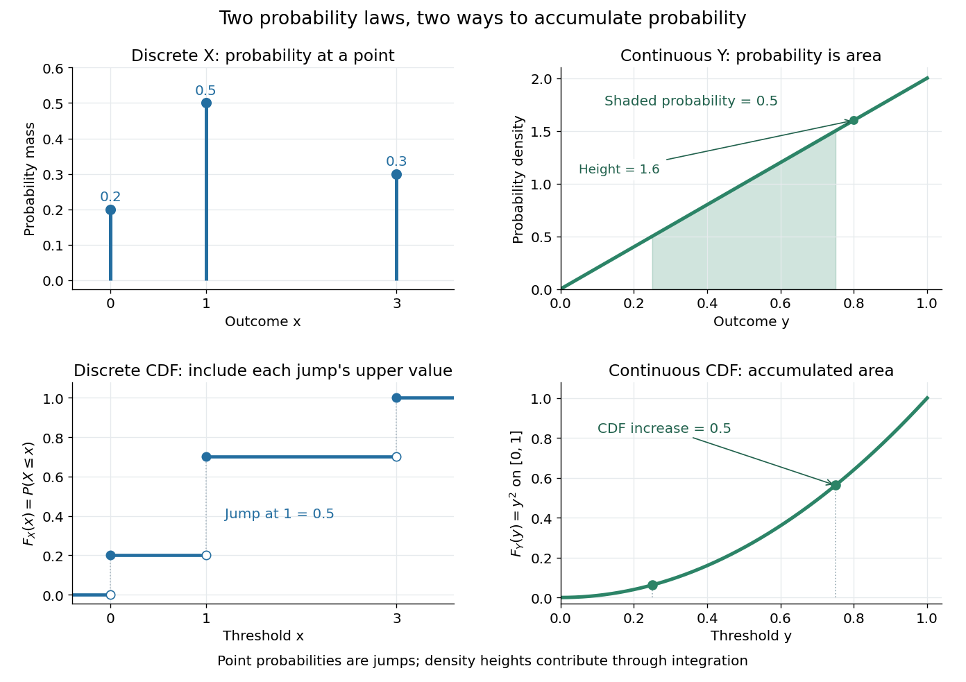
The cumulative distribution function answers all threshold questions for a real random variable, regardless of whether there are jumps or a probability density function. A quantile function reverses the direction of the question: given a cumulative probability level, find a threshold. This connects descriptive summaries to inverse transform sampling, which constructs a chosen probability distribution from a uniform distribution.

If $X$ has a continuous cumulative distribution function $F$, then $F(X)$ has the uniform distribution on $(0,1)$. Combined with inverse transform sampling, this constructs the monotone rearrangement $G^{-1}(F(X))$ to a target with quantile function $G^{-1}$.

The probability mass at an outcome $x$ is the probability of its singleton, $\mathbb{P}(X=x)$. It equals the jump $F_X(x)-F_X(x^{-})$ of the cumulative distribution function. For a discrete probability distribution these masses form the probability mass function; a continuous probability distribution gives every individual outcome mass zero. Positive probability mass at a point is distinct from the height of a probability density function.

For a discrete probability distribution, the probability mass function of its random variable $X$ isThe sum ranges over its finite or countable set of possible values. An event's probability is the sum of the masses of the included values. For the example under probability distribution, $\mathbb{P}(X\ge 1)=p_X(1)+p_X(3)=0.8$. The cumulative distribution function sums masses below a threshold; its jump at a value equals that value's probability mass. This differs from a probability density function, whose height is not a point probability.

If $q$ is the quantile function of an absolutely continuous probability distribution with probability density function $f$, then $q^{\prime }(u)=1/f(q(u))$ for almost every $u\in (0,1)$. Gaps in the support may give jumps in $q$, so the identity concerns its ordinary almost-everywhere derivative. It follows by differentiating the inverse relation to the cumulative distribution function.

The quantile function converts a cumulative probability level into a value. For a cumulative distribution function $F$ and $0<p<1$, use the generalized inverseIt selects the first threshold reaching the requested level. The infimum handles jumps and flat portions, so this construction does not require an ordinary inverse function. Other endpoint conventions are possible at $p=0$ or $p=1$; the open probability interval avoids those issues. NIST introduces the inverse-direction question as the percent point function. ^[ref].

For the finite example under probability distribution,Thus $Q_X(0.1)=0$, $Q_X(0.5)=1$, $Q_X(0.9)=3$. The value at $p=0.2$ is still zero, because $F_X(0)=0.2$ already reaches that level. For $F_Y(y)=y^2$ on $[0,1]$, the quantile function is $Q_Y(p)=\sqrt{p}$, giving $Q_Y(0.5)=1/\sqrt{2}\approx 0.70710678$.

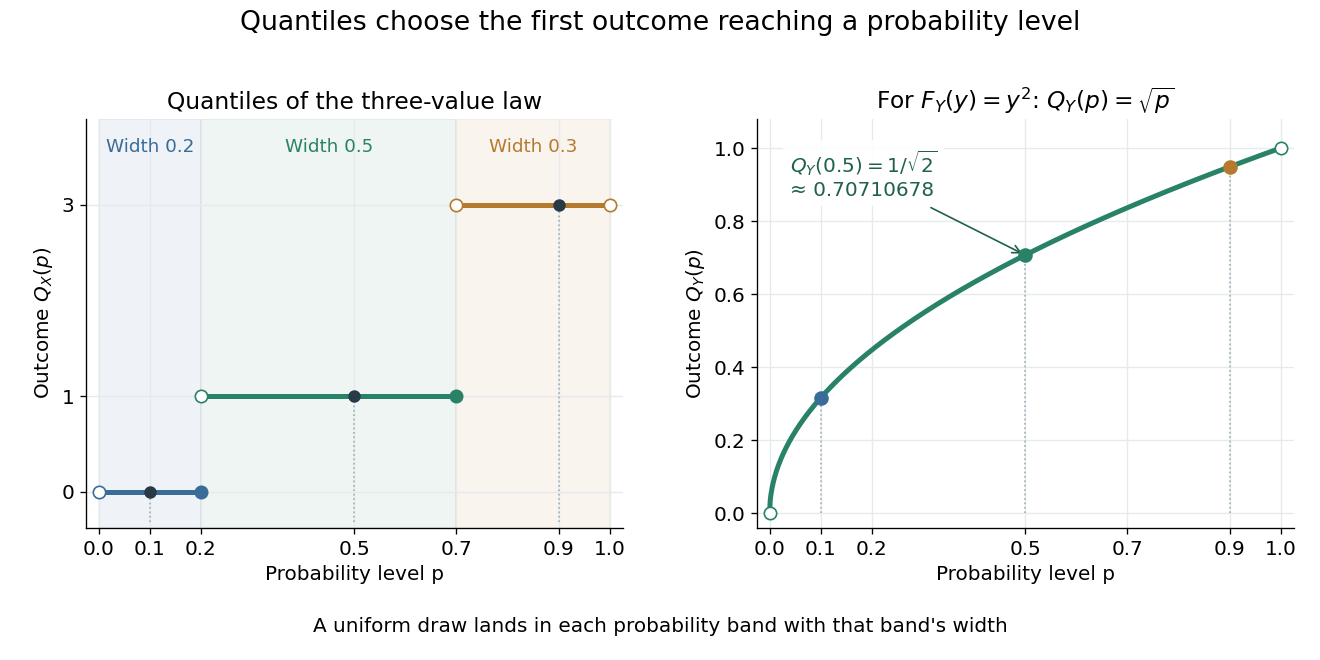
A median is a central threshold; $Q(1/2)$ supplies one, though a median need not be unique. The same quantile function becomes a sampling algorithm through inverse transform sampling. Jumps in $F$ become flat bands in $Q$, precisely the mechanism needed to assign positive probability to one outcome.

For a cumulative distribution function $G$, let $Q(u)=\inf \{x:G(x)\ge u\}$, $0<u<1$. Right continuity gives $Q(u)\le x$ exactly when $u\le G(x)$, including at atoms. Thus applying $Q$ to independent uniform variables $U_i$ constructs an independent sample with distribution function $G$. Its empirical distribution function is $G_n(x)=F_n(G(x))$, where $F_n$ is the uniform-sample empirical distribution function. Consequently ${\sup }_x|G_n(x)-G(x)|\le {\sup }_{t\in [0,1]}|F_n(t)-t|$. For the uniform sample, monotonicity and a grid of mesh $1/m$ bound the last supremum by the largest error at grid points plus $1/m$. The strong law of large numbers on the countable union of all such grids proves the almost-sure limit. This construction proves the theorem for distributions with atoms as well as continuous distributions.

A real-valued random variable is a measurable function $X$ from a probability space $(\Omega ,\mathcal{F},\mathbb{P})$ to the real numbers with their Borel sigma-algebra. More general targets give random elements. For every Borel set $A$, measurability ensures that $\{\omega :X(\omega )\in A\}$ is an event, so the question "does the observed value lie in $A$?" has a defined probability.

The function $X$ is fixed; its input outcome is uncertain. This separates what we measure from how the uncertainty is modeled. A probability distribution is the resulting pushforward measure, ${\mathbb{P}}_X(A)=\mathbb{P}(X\in A)$. A cumulative distribution function, probability mass function, or probability density function describes that measure in an appropriate setting. The random variable and its probability distribution are different objects: the former also retains its relationship to other measurements on the same sample space.

For two independent uniform dice, let $U,V$ record their results and define $S=U+V$ and $M=\max (U,V)$. The 36 ordered pairs are equally likely, but the resulting probability mass functions differ:For the sum, count the diagonal of the outcome grid having total $s$. For the maximum, subtract the $(m-1{)}^2$ pairs with both results below $m$ from the $m^2$ pairs with both results at most $m$. These examples show how a deterministic function transforms a simple input probability distribution into a nonuniform output one.

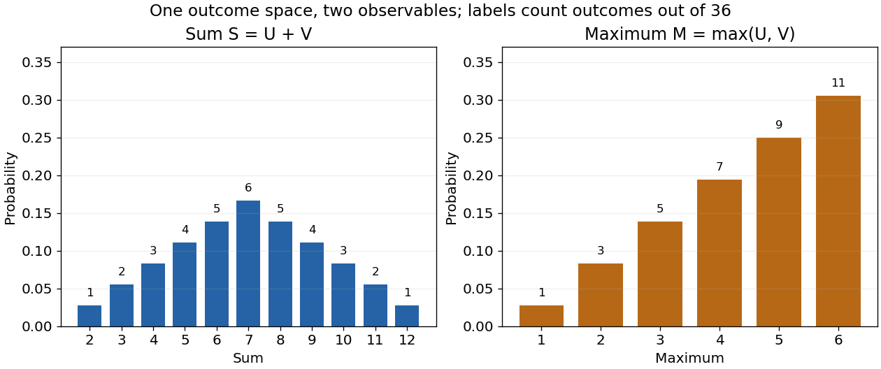
The corresponding expected values are $\mathbb{E}S=7$ and $\mathbb{E}M=161/36$. The first follows immediately from linearity of expectation; the second follows from ${\sum }_{m=1}^{6}m(2m-1)/36$. Neither number must be an attainable result. An expected value describes an average under the probability measure, not a prediction that the next observation will equal it.

The distinction between a random variable and its probability distribution matters for dependence. $U$ and $V$ have the same discrete uniform distribution and are independent random variables. $U$ and a second copy of $U$ also have that same marginal probability distribution, but they always agree. Their joint probability distribution is concentrated on the diagonal; the marginals alone cannot say which relationship holds. This is why a model for several measurements must specify their joint law or an appropriate independence assumption.

Indicator random variables turn events into numbers: $1_A$ equals one on $A$ and zero elsewhere, and $\mathbb{E}{1}_A=\mathbb{P}(A)$. This connects event counting with expected value and variance, and lets tools for random variables answer questions about probabilities. More complicated functions of observations can describe totals, waiting times, or estimation errors using the same framework.