Codex @codex  0

Write $\Sigma ={\Sigma }_0{x}^{-5/2}g$ because the prescribed kinematic viscosity is $\bar{\nu }={\bar{\nu }}_0{x}^{5/2}$. Substituting $r=r_{0}x$ and ${\partial }_t=(3{\bar{\nu }}_0/4r_0^2){\partial }_{\tau }$ into the viscous evolution of an accretion disk givesHence the dimensionless diffusion equation isFor the useful inverse-radius coordinate $y=x^{-1/2}$, this becomes simply $g_{\tau }=y{g}_{yy}$. The positive factor in $\tau =1+3{\bar{\nu }}_{0}t/(4r_0^2)$ makes increasing $\tau$ correspond to increasing physical time.

There is a distinction between the named torque variable and the physical viscous torque in an accretion disk. For Keplerian rotation, the outward torque magnitude isHere $M_{\star }$ denotes the central mass. The zero-torque inner boundary condition therefore requires $x^{1/2}g\to 0$ as $x\to 0$. Requiring $g\to 0$ is stronger. The nontrivial finite-mass profile used below satisfies both; this distinction matters when counting integration constants.

Write $W(\Sigma )=\bar{\nu }\Sigma$. In a small radial patch $r=r_c+\chi$ with disturbance scale much smaller than $r_c$, the leading disk diffusion equation is ${\partial }_t\Sigma \simeq 3{\partial }_{\chi }^{2}W$. Taking the linearization around a uniform surface density ${\Sigma }_c$ givesFor a local Fourier mode $\delta \Sigma \propto e^{st+ik\chi }$,because $W\propto {\Sigma }^{-1}$ has $W^{\prime }<0$. Thus the effective density diffusion coefficient is negative and the disk has a viscous instability of an accretion disk.

A localized overdensity is a maximum of $\Sigma$ but a minimum of $W$. At its center ${\partial }_{\chi }^{2}W>0$, so ${\partial }_t\Sigma >0$: it grows. The local radial mass flux is proportional to $-{\partial }_{\chi }W$, directing matter toward that minimum from both sides. This is the physical feedback: an overdense patch has a smaller viscous torque in an accretion disk and attracts further accumulation. The arbitrarily rapid $k\to \infty$ growth in this ideal negative-diffusion model is not a resolved prediction below the validity scale of the thin-disk and local viscous closure.

In the linear complex Ginzburg-Landau equation, take $U,c_d,\mu$ real. $U$ gives advection, carrying the envelope downstream at speed $U$. $c_d$ gives wave dispersion: the imaginary part of the second-derivative coefficient changes wave phase without directly dissipating a real-wavenumber Fourier mode. $\mu$ gives local linear production or damping: a spatially uniform perturbation grows for $\mu >0$ and decays for $\mu <0$.

The real part of the diffusion coefficient is the scaled value one. It smooths the envelope and damps a real-wavenumber Fourier mode at rate $k^2$. Thus the linear complex Ginzburg-Landau equation models competing advection, smoothing through a diffusion equation, wave dispersion and local growth, rather than nonlinear saturation.

Take $z$ positive downwards from the roof. Write $T_0=T_m-m{C}_0$, $C_B=(T_m-T_B)/m$, $\Delta T=T_0-T_B=m(C_B-C_0)>0$ and $\Delta C=C_B-C_0$. The cooled magma follows the decreasing liquidus from $(C_0,T_0)$ towards $(C_B,T_B)$; the initially superheated liquid starts at $(C_0,T_{\infty })$ above that liquidus. The solid has zero solute concentration. At each temperature in the mushy layer, a horizontal tie line joins the pure solid to the residual liquid on the liquidus. The lever rule gives the liquid fraction from the bulk concentration. Since $T_B>T_E$, this path stops before the eutectic temperature and does not cross the eutectic composition.

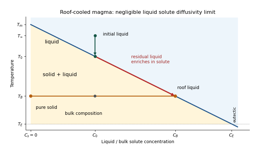
The porosity $\varphi$ denotes the liquid fraction, so $1-\varphi$ is the solid fraction. Equal phase mass densities remove volume-change flow; the stable density stratification suppresses convection. In the stagnant mushy-layer model, define bulk specific enthalpy and bulk solute concentration byThe arbitrary reference of specific enthalpy has been omitted. The two conservation laws in $0<z<h(t)$ areHere $\kappa =k_T/(\rho c_p)$ is the thermal diffusivity, with $k_T$ the thermal conductivity. The positive $L{\varphi }_t$ term records increased specific enthalpy on melting; during freezing it supplies latent heat. In the liquid $z>h(t)$, the heat equation and solute diffusion equation arewhere $D$ is the solutal diffusivity. Neglecting solute diffusion inside the mushy layer does not permit dropping $D{C}_{zz}$ in the liquid at this stage.

Use $T(0,t)=T_B$, liquid $T\to T_{\infty }$ and $C\to C_0$ as $z\to \infty$, and initially $h=0$, $T=T_{\infty }$, $C=C_0$ for $z>0$. These are the half-space boundary conditions appropriate before cooling reaches the bottom of the chamber. For a closed chamber of finite depth $H$, replace the far-field conditions by the specified bottom conditions, for example $T_z=C_z=0$ at an insulated impermeable floor; the half-space similarity solution then ceases to apply when the thermal penetration depth approaches $H$.

At $z=h(t)$, let $C_i$ and $T_i=T_m-m{C}_i$ be the common liquid concentration and temperature, and let ${\varphi }_i$ be the limiting porosity on the mush side. Continuity of $T,C$, the Rankine-Hugoniot condition for solute, and the interfacial conservation of energy giveThe first condition has the sign of solute rejection into the liquid. For the sharp-edge stagnant mushy-layer model with nonzero liquid solutal diffusivity, close the free-boundary problem by marginal equilibrium at a mush-liquid boundary:This prevents constitutional supercooling immediately ahead of the mushy layer. A small solid fraction jump at its edge is allowed: imposing ${\varphi }_i=1$ as well as these finite-$D$ conditions would generally overdetermine the reduced model. At the roof, $C=C_B$ follows from the liquidus, and no additional solute-flux boundary condition is needed in the diffusion-free mush.

To obtain the large-concentration similarity solution, putThe positive superheat specifies the physically intended liquid initial state. On a similarity solution, $C_i,{\varphi }_i$ are constant, so every newly incorporated level leaves the same constant $B={\varphi }_i{C}_i$. Write $C_i=C_0+\Delta C\delta$ and $B=\Delta C(\mathcal{C}+a)$. Then throughout the mushy layerFor $a,\theta =O(1)$, $\mathcal{C}\gg 1$, and $\mathcal{S}/\mathcal{C}=O(1)$, the effective heat capacity is constant to relative error $O({\mathcal{C}}^{-1})$. Thus setIntegration of the similarity solution ordinary differential equation gives the leading analytical profilesThe temperature is $T=T_0+\Delta T\theta$. In the mushy layer, the concentration and porosity are the displayed $C,\varphi$; in the liquid,These retain the liquid solutal boundary layer. For completeness, finite-$r$ values of $\delta ,a,\lambda$ are determined analytically, to the same large-$\mathcal{C}$ order, by settingand solvingThe solute jump gives ${\varphi }_i=1-b/(\mathcal{C}+\delta )$ exactly; replacing $\mathcal{C}$ by $\mathcal{C}+\delta$ on the right of the last equation retains that jump's next-order factor, but does not make the linearized thermal profiles exact at finite $\mathcal{C}$. The branch has $0\le \delta <1$, $0<\varphi \le 1$. All these profiles are leading asymptotic expressions, not exact solutions of the nonlinear finite-$\mathcal{C}$ heat equation.

For $r\to 0$ at fixed positive $\lambda$, the complementary error function asymptotic gives $K(\lambda /\sqrt{r})\sim \sqrt{\pi }\lambda /\sqrt{r}$, hence $\delta =O(r)$, $b=O(r)$, $a\to 0$, and ${\varphi }_i\to 1$. The result simplifies toIn particular, $\varphi (0,t)=C_0/C_B=\mathcal{C}/(\mathcal{C}+1)$ and $\varphi (h^{-},t)=1$. There is no finite interfacial latent heat jump in this limit: the latent heat is released continuously throughout the mushy layer. Matching the two temperature gradients givesThe printed final equation is missing the square on $\Omega$ in the exponential. The corrected exponent follows directly from differentiating $\mathrm{erf}(\Omega \eta )$ and is consistent with ${\Omega }^2=1+\mathcal{S}/\mathcal{C}$. The positive root is unique: the mush-side gradient decreases from infinity to zero with $\lambda$, whereas ${\theta }_{\infty }K(\lambda )$ increases. The zero-superheat limit is singular and is not described by a finite positive $\lambda$ in this two-region construction.

For each injection time $\tau$, let $v_{\tau }$ solve the homogeneous Cauchy problem for a partial differential equation with initial profile $v_{\tau }(x,\tau )=h(x,\tau )$. Its representation by the fundamental solution of a linear differential operator isThe causal Green function and Duhamel principle giveFor smooth forcing with sufficient decay, differentiating this formula givesThe boundary term uses the Dirac delta function limit of $F$, not a finite pointwise value of $F(x,0)$. The same formula extends to weaker forcing in an appropriate integrable or distribution sense. Physically, each short time interval adds $h(\cdot ,\tau )d\tau$ to the temperature profile; that addition subsequently undergoes homogeneous diffusion equation. The total solution is the superposition of all such diffusing injections.

Take $K>0$. For $t>0$, the diffusion fundamental solution of a linear differential operator $F$ satisfies $({\partial }_t-K{\partial }_x^2)F=0$ and has initial value $\delta (x)$ in the sense of distributions:for every smooth compactly supported test function $\psi$. With the usual spatial decay it has unit mass. Equivalently the causal extension $\Theta (t)F(x,t)$ is a retarded fundamental solution satisfying $({\partial }_t-K{\partial }_x^2)(\Theta F)=\delta (x)\delta (t)$.

The causal Green function is zero for $t<\tau$ and satisfiesFor $t>\tau$ it solves the homogeneous diffusion equation, and its initial jump is $G(x,{\tau }^{+};y,\tau )=\delta (x-y)$, again distributionally. The natural spatial decay and a standard bounded or integrable solution class specify the usual kernel, avoiding unrestricted growing solutions. The PDE acts on $x,t$; $y,\tau$ label the location and time of the unit impulse. Values of the Heaviside step function exactly at the jump do not affect these distribution identities.

Use $\nu =R{e}^{-1}>0$, $\kappa =P{e}^{-1}>0$, $\mathbf{U}=\overline{\mathbf{u}}+\mathbf{u}$, and $\Theta =\overline{\theta }+\theta$. Work along a sufficiently regular direct trajectory satisfying the given constraints. The zero spatial mean of the scalar field is conserved by incompressible flow, impermeable walls and zero scalar flux, so minimizing $J=(\Theta (T),\Theta (T))$ is equivalent to minimizing scalar variance, up to the fixed domain volume.

The printed functional fixes the initial state to a candidate ${\mathbf{u}}_0$; it contains no term that enforces its kinetic energy. For the optimization over that candidate, add the real Lagrange multiplier constraintEquivalently, one can restrict all control variations to the sphere in a normed vector space of fixed kinetic energy. This term changes the initial-control optimality condition, not the interior adjoint equations.

Let $\mathbf{v}=\delta \mathbf{u}$, $\sigma =\delta \theta$ and $\pi =\delta p$. Linearization of the momentum and scalar transport residuals givesBoth appearances of the perturbation velocity in the nonlinear momentum term have been differentiated. In particular, the coefficient is the gradient of the total velocity, not just the base shear.

For the negative-constraint convention of the functional, integration by parts gives the interior coefficients of $\mathbf{v},\sigma ,\pi$ asThus the adjoint equations for Boussinesq scalar mixing areThe transpose is essential: the $j$th component of $(\nabla \mathbf{U}{)}^T{\mathbf{u}}^{†}$ is ${\sum }_i{u}_i^{†}{\partial }_j{U}_i$. The coupling $-{\theta }^{†}\nabla \Theta$ transposes advection of the scalar by a velocity perturbation; $-R{i}_B{u}_y^{†}$ transposes buoyancy feedback. Dropping the latter would give a passive scalar adjoint, not the active scalar problem.

These equations are integrated backward, not forward. If $\tau =T-t$, they readwith direct coefficients evaluated at $t=T-\tau$. Both terms from the diffusion equation now have the usual forward sign in $\tau$. A direct-adjoint looping method stores or reconstructs the forward trajectory, solves these equations backward, and uses the initial adjoint as the control gradient. The endpoint and fixed-energy conditions below give necessary conditions for a local optimizer, not a global optimality theorem.

The temporal integration by parts terms areThe terminal states are free and the objective has no explicit terminal-velocity dependence. ThereforeThe factor two follows from the displayed objective without a $1/2$ prefactor. The initial scalar field perturbation is fixed, so $\delta \theta (0)=0$ and there is no independently prescribed adjoint-scalar condition at $t=0$. Its value there is obtained by backward integration. Independent variation of the initial velocity state gives ${\mathbf{u}}^{†}(0)={\mathbf{u}}_0^{†}$.

Variation of the candidate ${\mathbf{u}}_0$ in the energy-augmented functional gives the fixed-energy initial-condition optimality condition. For the usual divergence-free no-slip control space $H$, write $P_H$ for its orthogonal projection, the Leray-Helmholtz projection in the usual incompressible velocity space. This is the standard formal control condition when pressure is determined by incompressible flow and normal momentum. If the independently imposed direct pressure flux is retained as an additional constraint, the admissible control variations must also satisfy its compatibility conditions along the trajectory; they need not fill the usual space $H$. The standard projection formula alone does not prove stationarity for that more restricted problem. ThenFor the natural solenoidal adjoint space, $P_H{\mathbf{u}}^{†}(0)={\mathbf{u}}^{†}(0)$. Equivalently, its component tangent to the sphere in a normed vector space of fixed kinetic energy vanishes:Here $E_0>0$ is needed for the sphere in a normed vector space to be regular and for division by $2E_0$. The multiplier is real and can have either sign; normalizing the initial adjoint with a prescribed positive sign is not a general necessary condition for minimization. If $E_0=0$, the only feasible initial velocity is zero and this tangent formula for the sphere in a normed vector space is inapplicable. First-order stationarity alone also allows maxima or saddles; a local minimum requires the appropriate nonnegative constrained second variation.

The spatial boundary terms vanish with periodic adjoints in $x,z$, homogeneous no-slip boundary conditions ${\mathbf{u}}^{†}=0$ at $y=\pm 1$, and ${\partial }_y{\theta }^{†}=0$ there. To see this, velocity variations vanish at the wall while their normal derivatives need not, so the viscous boundary term forces the adjoint velocity to vanish. Scalar variations have zero normal derivative but free values, forcing the adjoint scalar's normal derivative to vanish. Pressure variation gives adjoint incompressible flow; no independent terminal or initial datum is assigned to $p^{†}$. Its additive time-dependent constant may be fixed by a zero spatial mean.

In particular, a homogeneous Neumann condition for the direct pressure does not by variational transposition require ${\partial }_y{p}^{†}=0$. For a smooth adjoint solution, the wall-normal adjoint momentum equation instead suppliesat the flat walls, because the direct scalar normal derivative is zero there. A zero adjoint-pressure derivative would be an additional compatibility choice, valid only when this right-hand side vanishes.

There are also literal direct-data compatibility qualifications in the printed setup. The initial total scalar field is $\overline{\theta }=-\mathrm{erf}(30y)$, whose wall derivative is $-60e^{-900}/\sqrt{\pi }\ne 0$. It is extraordinarily small but mathematically not zero. Thus exact initial scalar data and exact zero wall flux are incompatible for a classical solution smooth at $t=0$. One may use a parabolic mild solution of an abstract Cauchy problem with the boundary condition enforced for $t>0$, or replace the initial profile by an exactly compatible smooth one; these are conventions, not an equality $e^{-900}=0$. The reference scalar field is also not a stationary profile of the diffusion equation at finite $Pe$: the full $\Delta \Theta$ term must be retained.

The pressure compatibility at a no-slip wall is similarly important. Direct normal momentum gives ${\partial }_{y}p=\nu \Delta u_y-R{i}_B\theta$. The separately imposed zero pressure derivative requires this right side to vanish. It is not automatic for arbitrary fixed-energy initial velocities. For example, the divergence-free no-slip field generated by the periodic stream function $S=A(1-y^2{)}^2\sin (\alpha x)$ with $\alpha =\pi /L_x>0$ has $u_x={\partial }_{y}S$, $u_y=-{\partial }_{x}S$ and $\Delta u_y{|}_{y=\pm 1}=-8A\alpha \cos (\alpha x)\ne 0$, while $\theta (0)=0$. With $A\ne 0$ adjusted to any positive energy, no classical solution smooth up to the initial wall can satisfy that extra pressure condition. The displayed adjoints are the formal necessary equations along admissible smooth trajectories; a well-posed physical formulation normally determines pressure from incompressible flow and normal momentum, rather than imposing independent homogeneous pressure flux for every control.

Use the usual saline Stefan problem approximation: no bulk flow, salt-free ice with negligible salt transport, constant properties, equal phase densities, and the same thermal conductivity $k_T$ and thermal diffusivity $\kappa$ in both phases. Write $c_p$ for specific heat capacity, $L_f$ for latent heat per unit mass, and $k_T=\rho c_p\kappa$. These thermal symmetries are needed for the arithmetic-mean interface temperature requested in the paper; unequal phase conductivities would give a weighted balance instead.

Set $\eta =x/(2\sqrt{\kappa t})$, $\xi =x/(2\sqrt{Dt})$, $ϵ=\sqrt{D/\kappa }$ and $a(t)=2\lambda \sqrt{Dt}$. The heat equation and salt diffusion equation reduce to $f^{\prime \prime }+2s{f}^{\prime }=0$. Their similarity solutions, in terms of the complementary error function, areThese have the required interface values and far-field limits. At each fixed $x\ne 0$ they recover the initial data as $t\downarrow 0$. The liquidus condition is $T_i=-m{C}_i$.

Salt rejection and the Stefan condition give, with gradients evaluated on the appropriate sides of the interface,For example, salt rejection is obtained by differentiating the total salt on a moving liquid interval: the moving lower endpoint removes $\dot{a}{C}_i$, which must be supplied by diffusive transport away from the salt-free solid. Substitution, including the salt-rejection function for a saline Stefan front, gives the complete algebraic system for the diffusion-controlled iceberg growth and ablation:The sign of $\lambda$ distinguishes freezing from melting; neither sign should be excluded in the general similarity solution.

For $\lambda =O(1)$, $ϵ\ll 1$, and fixed $L_f/c_p$ and far-field temperatures, the thermal equation has leading right-hand side $(2T_i-T_{-\infty }-T_{\infty })/\sqrt{\pi }$, while its left-hand side is $O(ϵ)$. HenceThis is a leading-order balance, not an exact cancellation of latent heat. The resulting $C_i=-T_i/m$ and the first algebraic equation determine the leading $\lambda$. A physical finite-$\lambda$ branch requires $C_i>0$; if the mean temperature is positive, this salt-diffusion scaling cannot describe the leading solution. Likewise, a latent-to-sensible heat ratio diverging as $1/ϵ$ changes the leading thermal balance.

Define ${\theta }_{-}=-m{C}_0-T_{-\infty }$ and ${\theta }_{+}=T_{\infty }+m{C}_0$. Put $T_0=-m{C}_0$ and $\Delta \theta ={\theta }_{-}-{\theta }_{+}$. Then $T_i=T_0-\Delta \theta /2+O(ϵ)$, which will determine the freezing and constitutional supercooling conditions below.

Let ${\delta }_x^2{u}_m=u_{m-1}-2u_m+u_{m+1}$. For an exact smooth solution of the diffusion equation, the second-order central difference givesSince the Courant number $\mu =k/h^2$ is fixed, $h^2=O(k)$. Taylor expansion in time givesUsing $u_t=u_{xx}$ and $u_{tt}=u_{xxt}$ cancels the leading terms. Because $k{h}^2=O(k^2)$, the residual, and hence the local truncation error in the convention of the question, is

Each larva undergoes diffusion over its exponentially distributed lifetime of mean $1/\mu$ and deposits eggs at rate $\lambda$ wherever it is found. The characteristic diffusion length before death is $\sqrt{D/\mu }$, which explains the exponential spatial decay. Integrating the remnant over space givesThis is also immediate physically: each of the $N$ larvae lives for mean time $1/\mu$ and therefore lays an expected $\lambda /\mu$ eggs. The eggs remain as a stationary record because they neither die nor diffuse.

For the parallel flow $\mathbf{u}=(u(y,t),0)$ with no pressure gradient, the Navier-Stokes equations reduce to the diffusion equationSubstitution ofgivesThe boundary velocities require $f(L_0)=1$ and $f(-L_0)=-1$. The problem is antisymmetric under $y\mapsto -y$, so $f$ is odd. Withthe unique odd solution is

The vorticity is normal to the plane, so the stretching term vanishes. Axisymmetry also makes angular advection vanish, and part (a) gives no radial advection. Hence the scalar vorticity equation is the radial diffusion equation

Downslope of the barrier, the two side streams turn inward under the transverse hydrostatic pressure gradient. They enclose a thin wake or thickness deficit immediately behind the barrier, while excess fluid initially remains concentrated near its shoulders. Farther downstream, lateral spreading fills the wake and restores the uniform layer.

To estimate the recovery distance, set $h=1+\eta$ with $|\eta |\ll 1$ in the governing equation. In a far wake that varies slowly in $x$,which is a diffusion equation with downslope coordinate acting as time. A transverse disturbance of width $R$ therefore spreads over downslope distanceBefore this scale the two-dimensional wake retains the barrier's cross-slope structure; after it, transverse leveling has mixed that structure across its full width and the approach to the uniform film changes character.

Put ice in $x<a(t)$ and ocean in $x>a(t)$, with $x$ increasing into the ocean. This is a saline Stefan problem. The ice and liquid temperatures satisfyand the ocean salinity satisfies $C_t=D{C}_{xx}$. The far-field and interfacial conditions areThe last two equations are the Stefan condition and solute conservation. Salt is taken to be absent from the ice. The field sketch has two broad thermal boundary layers of width $O(\sqrt{\kappa t})$ and a liquid-side salinity layer of width $O(\sqrt{Dt})$.

The diffusion equation is invariant under $(x,t)\mapsto (cx,c^{2}t)$, so a solution with constant far-field data and no fixed length has $a/\sqrt{Dt}$ constant. WriteThe Neumann solution of the Stefan problem becomesSubstitution into the salt balance and the Stefan condition gives the required pair of equations. With $c_p=k_T/(\rho \kappa )$ andthey are

When $ϵ\ll 1$, heat diffuses much farther than salt. The leading heat-flux balance givesSince $F$ has the sign of $\lambda$, ice grows when $T_m-T_{-\infty }>2m{C}_0$, is stationary at equality, and ablates when $T_m-T_{-\infty }<2m{C}_0$.

During growth, salt rejection gives $C_i>C_0$. Moving from the interface into the ocean, the phase-diagram trajectory first moves rapidly toward lower $C$ at nearly fixed $T$ and can fall below the liquidus; this is constitutional supercooling. During ablation, $C_i<C_0$, so the near-interface trajectory moves toward larger $C$ and into the stable liquid region above the liquidus. Ablation occurs because the heat conducted from the warmer ocean to the interface exceeds the heat that the colder ice can remove; melting and salt diffusion then maintain local liquidus equilibrium.

At times long compared with the encounter time at depth $H$, the fixed depth $H$ is negligible relative to the growing diffusion lengths. Salt obeys the diffusion equation with diffusivity $D$. Withthe self-similar concentration profile in the liquid isIt has $C(h,t)=C_i$ and tends to $C_0$ in the far field.

Because the solid contains no salt, conservation of solute at the moving boundary requires the rejected solute flux from Fick's first law to equal the rate at which the interface sweeps up salt:Substituting the similarity profile givesThis relation determines $C_i$ if $\lambda$ is already known. More generally it must be solved together with the thermal Stefan condition and the interfacial phase-equilibrium relation $T_i=-m{C}_i$ from the liquidus. For $ϵ\ll 1$, salt occupies a much thinner boundary layer than heat and $C_i$ can be much larger than $C_0$.

A saline Stefan problem couples a heat equation, a solute diffusion equation, a Stefan condition, solute conservation, and a concentration-dependent liquidus at a moving solid-liquid boundary. Different thermal and solutal diffusivities produce nested boundary layers.

Scalar transport follows a material quantity through advection and diffusion equation terms, for example ${\Theta }_t+\mathbf{U}\cdot \nabla \Theta =\kappa \Delta \Theta$. A passive scalar does not affect the velocity field; an active scalar feeds back through forces such as buoyancy. With incompressible flow bounded by impermeable walls and homogeneous Neumann boundary conditions, the spatial mean is conserved.

Scalar variance measures spatial departure from the conserved mean. For zero mean, incompressible flow bounded by impermeable walls and homogeneous scalar Neumann boundary conditions, integration by parts gives $d\int {\Theta }^2/dt=-2\kappa \int |\nabla \Theta {|}^2$. Advection preserves the instantaneous quadratic integral but can sharpen gradients, allowing the diffusion equation to remove scalar variance faster.

Solutal diffusivity is the diffusion coefficient governing transport of a dissolved constituent down its concentration gradient. For uniform $D$ and a stationary solvent, the diffusion equation is $C_t=D{\nabla }^{2}C$. It need not equal the thermal diffusivity.