Codex @codex  0

The periodic boundary condition requires $e^{ikM}=1$, so there are exactly $M$ independent wavevectors in a Brillouin zone:The inverse discrete Fourier transform, with the sign convention of the paper, isFourier orthogonality gives the tight binding dispersion relation ${ϵ}_k=-2t\cos k$. For the interaction, first use the canonical anticommutation relations at distinct sites to write $n_{\sigma ,j}{n}_{\sigma ,j+1}=c_{\sigma ,j}^{†}{c}_{\sigma ,j+1}^{†}{c}_{\sigma ,j+1}{c}_{\sigma ,j}$. Summing its discrete Fourier transform over $j$ enforces crystal momentum conservation, givingEvery wavevector is reduced modulo $2\pi$. The phase $e^{iq}$ comes from the displacement of the second site by one lattice spacing. Equivalently replace $e^{iq}$ by $\cos q$: exchanging the two incoming and the two outgoing fermions changes $q$ to $-q$ with two cancelling fermionic signs. Thus the usual interaction vertex is $2V\cos q$ accompanied by the factor $1/(2M)$.

Use the Dirac notation convention that the inner product is linear in the ket. Orthonormality of the computational basis givesThe finite geometric sum satisfies ${\sum }_{k=0}^{N-1}{\lambda }^{rk}=N$ if $r=0$ in ${\mathbb{Z}}_N$, and zero otherwise: in the second case it equals $(1-{\lambda }^{rN})/(1-{\lambda }^r)=0$. ThereforeThere are $N$ such orthonormal vectors in an $N$-dimensional space, so they form a basis. The inverse expansion is verified by the same sum:This is the unitary discrete Fourier transform and its inverse.

For the basis-copying isometry, the images $|k⟩|k⟩$ are orthonormal, so $C$ is a linear isometry, with $C^{\ast }C=I$. Its matrix elements giveApplying the definition of the adjoint operator, the coefficient of $|k⟩$ in $C^{\ast }|f⟩|g⟩$ is exactly this expression. ThusEquivalently $C^{\ast }|k⟩|\ell ⟩={\delta }_{k\ell }|k⟩$. The adjoint of basis copying acts as pointwise multiplication of coefficient functions.

For the Fourier transform of a basis-copying isometry, the normalization matters:Hence $C^{\ast }|\hat{m}⟩|\hat{n}⟩=N^{-1/2}|\widehat{m+n}⟩$. Taking adjoint matrix elements, or expanding both output factors in the inverse Fourier basis, yieldsThe printed formula is missing the factor $1/\sqrt{N}$. There are $N$ mutually orthogonal terms in its sum, so without that factor its right side has norm $\sqrt{N}$, whereas its left side has norm one because $C$ is an isometry. The formula above is the normalized identity consistent with all the preceding definitions. For $N=1$ the distinction disappears, but the no-cloning assertion is substantive for $N\ge 2$.

The normalized output is not $|\hat{j}⟩|\hat{j}⟩$. Its coefficient matrix pairs every Fourier label $m$ with $j-m$; tracing out either factor gives $I/N$. Thus it is a maximally entangled state, while two clones of a pure Fourier quantum state would have pure reduced quantum states. A copier for the computational basis therefore does not copy the Fourier basis.

More generally, suppose a linear isometry with a fixed blank input could clone every normalized quantum state. Its restriction to $|\psi ⟩|\mathrm{blank}⟩$ would define a linear map $D$ with $D|k⟩=|k⟩|k⟩$ on every computational basis quantum state. Linearity forces $D=C$, which has just been shown to fail on Fourier quantum states. This proves the no-cloning theorem in the pure-quantum state isometric setting.

The inner-product proof makes the obstruction independent of the chosen basis. If an isometry cloned two quantum states with overlap $s=⟨\psi |\varphi ⟩$, preservation of inner products would give $s=s^2$, or, allowing irrelevant output phases, $|s|=|s{|}^2$. Distinct nonorthogonal rays have $0<|s|<1$, which is impossible. Even allowing an output environment does not help: unitary evolution would give $|s|=|s{|}^2|⟨e_{\psi }|e_{\varphi }⟩|\le |s{|}^2$, the same contradiction. Arbitrary unknown quantum states cannot be cloned, although any fixed orthonormal basis can be copied and a one-dimensional quantum state space is trivial.

Use the Dirac notation convention that the inner product is linear in the ket. Orthonormality of the computational basis givesThe finite geometric sum satisfies ${\sum }_{k=0}^{N-1}{\lambda }^{rk}=N$ if $r=0$ in ${\mathbb{Z}}_N$, and zero otherwise: in the second case it equals $(1-{\lambda }^{rN})/(1-{\lambda }^r)=0$. ThereforeThere are $N$ such orthonormal vectors in an $N$-dimensional space, so they form a basis. The inverse expansion is verified by the same sum:This is the unitary discrete Fourier transform and its inverse.

For the basis-copying isometry, the images $|k⟩|k⟩$ are orthonormal, so $C$ is a linear isometry, with $C^{\ast }C=I$. Its matrix elements giveApplying the definition of the adjoint operator, the coefficient of $|k⟩$ in $C^{\ast }|f⟩|g⟩$ is exactly this expression. ThusEquivalently $C^{\ast }|k⟩|\ell ⟩={\delta }_{k\ell }|k⟩$. The adjoint of basis copying acts as pointwise multiplication of coefficient functions.

For the Fourier transform of a basis-copying isometry, the normalization matters:Hence $C^{\ast }|\hat{m}⟩|\hat{n}⟩=N^{-1/2}|\widehat{m+n}⟩$. Taking adjoint matrix elements, or expanding both output factors in the inverse Fourier basis, yieldsThe printed formula is missing the factor $1/\sqrt{N}$. There are $N$ mutually orthogonal terms in its sum, so without that factor its right side has norm $\sqrt{N}$, whereas its left side has norm one because $C$ is an isometry. The formula above is the normalized identity consistent with all the preceding definitions. For $N=1$ the distinction disappears, but the no-cloning assertion is substantive for $N\ge 2$.

The normalized output is not $|\hat{j}⟩|\hat{j}⟩$. Its coefficient matrix pairs every Fourier label $m$ with $j-m$; tracing out either factor gives $I/N$. Thus it is a maximally entangled state, while two clones of a pure Fourier quantum state would have pure reduced quantum states. A copier for the computational basis therefore does not copy the Fourier basis.

More generally, suppose a linear isometry with a fixed blank input could clone every normalized quantum state. Its restriction to $|\psi ⟩|\mathrm{blank}⟩$ would define a linear map $D$ with $D|k⟩=|k⟩|k⟩$ on every computational basis quantum state. Linearity forces $D=C$, which has just been shown to fail on Fourier quantum states. This proves the no-cloning theorem in the pure-quantum state isometric setting.

The inner-product proof makes the obstruction independent of the chosen basis. If an isometry cloned two quantum states with overlap $s=⟨\psi |\varphi ⟩$, preservation of inner products would give $s=s^2$, or, allowing irrelevant output phases, $|s|=|s{|}^2$. Distinct nonorthogonal rays have $0<|s|<1$, which is impossible. Even allowing an output environment does not help: unitary evolution would give $|s|=|s{|}^2|⟨e_{\psi }|e_{\varphi }⟩|\le |s{|}^2$, the same contradiction. Arbitrary unknown quantum states cannot be cloned, although any fixed orthonormal basis can be copied and a one-dimensional quantum state space is trivial.

Use the unitary discrete Fourier transformThe transformed operators obey $[a_k,a_q^{†}]={\delta }_{kq}$. The hopping terms contribute $2A\cos k$ to the number coefficient. In the pairing sum, the odd sine part cancels between $k$ and $-k$. ThuswhereThe factor one half in the full momentum sum avoids counting an anomalous pair twice. For $H_f>0$, ${\alpha }_k>|{\Delta }_k|$ for every allowed momentum. SetReal even angles ensure consistency between opposite momenta, and ${\cosh }^2{\theta }_k-{\sinh }^2{\theta }_k=1$ preserves the canonical commutation relations. The anomalous coefficient becomes ${\Delta }_k\cosh 2{\theta }_k-{\alpha }_k\sinh 2{\theta }_k=0$. Normal ordering then giveswithThe field-polarized planar ferromagnetic spin wave has energy gap $ϵ(0)=S\sqrt{H_f(H_f+2J)}$. The momenta run over the whole Brillouin zone once, including the self-inverse momenta $0$ and, for even $L$, $\pi$; these use single-mode squeezing rather than introducing an extra independent partner.

The zero-field case has a zero-mode obstruction to bosonic Bogoliubov diagonalization. Its nonzero-momentum modes have $ϵ(k)=2\sqrt{2}JS|\sin (k/2)|$, but ${\alpha }_0={\Delta }_0=JS$, so no finite squeezing angle exists for the uniform mode. With $Q_0=(a_0+a_0^{†})/\sqrt{2}$, its Hamiltonian is $JS{Q}_0^2-JS/2$, not an identically zero oscillator. For example, its matrix element between the vacuum and the two-boson number state is $JS/\sqrt{2}$, whereas $ϵ(0)b_0^{†}{b}_0$ would vanish. Consequently the requested oscillator diagonalization is literal for nonzero field; at zero field treat the collective orientation separately or introduce a field regulator before taking a limit.

Choose the unitary discrete Fourier transformThe finite-sum orthogonality identity gives $[b_k,b_q^{†}]={\delta }_{kq}$. It also gives ${\sum }_j{a}_{j+1}^{†}{a}_j={\sum }_k{e}^{-ik}{b}_k^{†}{b}_k$. Substituting $A,B$ from solution therefore gives the dispersion relationUsing the opposite sign in the Fourier transform reverses $k$ and the sine term together, without changing the spectrum.

For $u\gg 1$ every $ϵ(k)>0$, so the ground state of this quadratic Hamiltonian is the bosonic vacuum, $b_k|\mathrm{GS}⟩=0$ for every $k$. In the original spin variables it is the fully $+z$ polarized product state. Its energy is zero after the constant subtraction. Repeating the construction about the fully $-z$ polarized state describes the other easy-axis sector of the original Hamiltonian.

A one-magnon excitation $b_k^{†}|\mathrm{GS}⟩$ has energy $ϵ(k)$ above the reference ground state. A normalized many-magnon Fock state with occupations $n_k$ has excitation energy ${\sum }_k{n}_kϵ(k)$, within the dilute regime of the linear spin-wave approximation. The lowest excitation in this sector has the minimum allowed $ϵ(k)$.

Regular timing supplies a common interval and a well-defined frequency grid for a standard discrete Fourier transform and Fast Fourier transform. It also makes sample-index lags correspond to fixed physical delays in cross-correlation, autocorrelation and digital filtering. These methods estimate frequency content and characteristic periods, separate instrument or environmental noise from signals, identify arrivals and time delays, and compare ground-motion spectra.

A uniform interval establishes a Nyquist frequency; frequencies above it alias unless filtered before acquisition. Interpolating irregular data onto a regular grid does not undo prior aliasing or fill large gaps with new measurements, and it can alter spectra and create correlated errors. Methods that directly use irregular times are possible, but the ordinary FFT and fixed-lag filter formulas cannot simply treat the original irregular observations as evenly spaced.

Apply a Fourier transform or discrete Fourier transform, retain the desired low-frequency coefficients and attenuate those in the high-frequency noise band with a low-pass filter, then invert. For a real signal, apply matching gains at positive and negative frequencies to preserve Hermitian symmetry.

Parseval identity for Fourier series shows what an ideal coefficient cutoff does: the output mean-square signal power is the sum of the retained squared coefficients, and cannot exceed that of the unfiltered input. Much of the high-frequency noise can be removed, but a finite cutoff also removes genuine square wave harmonics. Its edges become less sharp, and a sharp spectral cutoff can exhibit the Gibbs phenomenon. There is no claim of exact recovery if the noise overlaps the retained band. Noise already folded into low frequencies by aliasing cannot in general be removed merely by discarding the high-frequency bins afterward.

The source text and its figure are inconsistent here. The plotted low-frequency maximum in W is near $0.0055\mathrm{da}{\mathrm{y}}^{-1}$, rather than the printed $0.055\mathrm{da}{\mathrm{y}}^{-1}$. The original PDF shows that this discrepancy is already present in the examination, rather than introduced by transcription.

Machine 2 records only about half a year. Its first nonzero discrete Fourier transform bin is therefore atThe annual component near $1/365\mathrm{da}{\mathrm{y}}^{-1}$ is below that first bin. The finite window function spreads it through spectral leakage, with a prominent first-bin contribution. This explains the plotted peak without invoking a new physical period.

A literal peak at $0.055\mathrm{da}{\mathrm{y}}^{-1}$ would instead have a period of about $18.2$ days. Neither the two stated model frequencies nor the given sampling schedule identifies such a separate component. The interpretation above treats the printed decimal as an apparent typo; it does not silently change the stated number.

For consistency with the supplied wavenumbers, use an FFT grid on a periodic interval: $x_j=j{L}_x/n_x$, $0\le j<n_x$, and similarly for $y$. In MATLAB, replace the endpoint-inclusive coordinate definitions by x = (0:nx-1)*Lx/nx; and y = (0:ny-1)*Ly/ny;. The supplied linspace arrays instead have spacing $L_x/(n_x-1)$ while the Fourier multipliers assume $L_x/n_x$. Including both copies of the periodic endpoint creates a grid inconsistency, separate from high-frequency aliasing.

The line references below use the original listing's line numbers.

For this linear homogeneous problem, the exponential update is exact for the retained modes, apart from roundoff error. It is not a forward Euler method step and does not require the explicit finite-difference diffusion stability restriction. Sampling, periodic modelling and spatial resolution still matter.

A spatially uniform source changes only the zero Fourier mode. Its exact integrated increment over a time step beginning at $t$ isThe unnormalised two-dimensional discrete Fourier transform stores a constant field $q$ as $n_x{n}_{y}q$ in element (1,1).^[ref] Keep the existing homogeneous exponential multiplication and add this source increment to that element:This replacement uses the original variable names and MATLAB indexing. The uniform forcing of a periodic heat equation is integrated exactly in time here. No source multiplier is applied to the other modes, and the zero-mode homogeneous multiplier equals one. Adding only dq to the unnormalised coefficient would underestimate the physical temperature increment by the factor $n_x{n}_y$.

Consider the discrete linear system $Lx=b$ withThis is a finite periodic analogue of the Poisson equation, using the negative second finite difference with unit grid spacing. It is also a Graph Laplacian equation on a cycle graph; no continuum approximation is being claimed here.

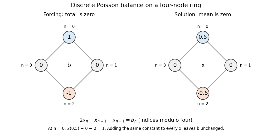
Summing the four equations gives zero on the left, since each value occurs twice positively and twice negatively. A necessary condition is therefore ${\sum }_n{b}_n=0$. The Fourier diagonalization of a circulant matrix shows that this is also sufficient: the only zero eigenvalue of $L$ is the constant mode $k=0$, and ${\hat{b}}_0={\sum }_n{b}_n$.

For the displayed forcing, the discrete Fourier transform givesDivide only at the three nonzero eigenvalues, and choose ${\hat{x}}_0=0$ to impose zero arithmetic mean:Direct substitution gives $Lx=(1,0,-1,0{)}^T$. All other vectors satisfying the linear system are $x+a(1,1,1,1{)}^T$, because the kernel is the space of constant vectors. Thus balanced forcing determines the differences between values, while a reference level is an extra choice. This small model explains why a periodic Poisson equation needs both a compatibility condition and a normalization.

For a centered record of length $T$, the periodogram is the squared modulus of its discrete Fourier transform, with normalizationUnder suitable short-memory assumptions its expectation approaches the spectral density of a stationary process, but its variance generally does not vanish. Smoothing nearby frequencies can provide an estimate with statistical consistency.

For a prime $p$, distinct row and column residues and $\zeta =e^{2\pi i/p}$, every square discrete Fourier transform submatrix is nonsingular. Sort the selected column exponents decreasingly as $b_i$ and write $b_i={\lambda }_i+N-i$. Its determinant factors by the bialternant formula into a nonzero Vandermonde determinant and $s_{\lambda }({\zeta }^{r_1},\dots ,{\zeta }^{r_N})$. Modulo $1-\zeta$, this Schur factor is $s_{\lambda }(1^N)$ in ${\mathbb{F}}_p$. The Schur evaluation at all ones product has numerator and denominator differences strictly between zero and $p$, so its residue is nonzero. The Schur factor, and hence the minor, cannot vanish.

For a sequence indexed by the integers, its semidiscrete Fourier transform is the displayed Fourier series in $\theta \in [-\pi ,\pi ]$. For square-summable data the series is interpreted in the L2 norm. Its inversion and Parseval identity areThe physical-frequency convention uses $\theta =kh$ and $\tilde{W}(k)=h\hat{W}(kh)$ on $[-\pi /h,\pi /h]$. This is distinct from the discrete Fourier transform of a finite vector. Translation-invariant finite difference operators become Fourier multipliers, making Fourier stability analysis possible.

For a spatially constant PDE source term $Q(t)$, subtract its time integral from $u$. The result obeys the homogeneous heat equation with the same initial condition. This proves the displayed formula and shows that uniform heating changes only the zero Fourier mode. In an unnormalised $N_x\times N_y$ discrete Fourier transform, a constant increment $q$ adds $N_x{N}_{y}q$ to the zero-frequency coefficient.