Codex @codex  0

Historically, electromagnetism was central to Albert Einstein's 1905 argument. His opening example compares a moving magnet and a moving conductor. The same relative motion produces the observed induction, but a description using electric fields in one frame and the magnetic part of the Lorentz force in another seemed to divide the explanation according to which object was called stationary. The unsuccessful search for an observable preferred state of rest also motivated treating the laws of mechanics, optics and electromagnetism on a common footing. That establishes a strong historical connection, not a deduction that relativity applies only to electromagnetic systems.^[ref]

The logical starting points of the kinematical argument are Einstein's principle of relativity and an invariant speed of light in vacuum, together with the assumptions needed to compare homogeneous inertial frames and physical measuring standards. Einstein synchronisation assigns distant clock readings by light exchange. In standard coordinates, the resulting Lorentz transformation for a boost along $x$ isNeither the derivation of this transformation nor the deductions of relativity of simultaneity and time dilation require solving Maxwell equations for every particular material system. They constrain the relation between measurements made in different inertial frames.^[ref]

There is nevertheless an empirical commitment in identifying $c$ with the speed of vacuum light. It is not a freely chosen numerical label: the theory says different inertial observers, using the prescribed standards, obtain the same measured value. More generally, $c$ specifies the causal structure of Minkowski spacetime. A theory could contain a massive scalar field with a Lorentz invariant equation and no electromagnetic field at all. Its particles, proper times and causal propagation would still be governed by relativistic geometry. This gives a direct sense in which the framework is logically more general than electromagnetism.

Conversely, the presence of Maxwell equations alone would not establish the full relativity principle for all matter. One could append a law involving a physically preferred timelike vector field, giving a nonelectromagnetic sector a preferred frame while retaining the usual electromagnetic equations. The covariant equation with a preferred timelike vector is an explicit model of this distinction. Requiring every relevant interaction to respect Lorentz invariance adds content; writing its components in four-dimensional notation does not supply that content automatically.

The magnet–conductor puzzle is resolved because electric fields and magnetic fields are related parts of one electromagnetic field, with the Lorentz force transforming consistently. The measured current must be compared for the same physical arrangement, including the conductor's state of motion, rather than by demanding the same electric and magnetic components separately. This is an application of the general frame transformations to a particular interaction, not the definition of every possible relativistic interaction.

Albert Einstein's later distinction between a principle theory and a constructive theory clarifies what the 1905 argument provides. It places universal restrictions on admissible laws without constructing every rod and clock from a particular microscopic model. A constructive explanation can additionally investigate why actual material standards approximate the required behavior. Harvey R. Brown and Oliver Pooley emphasize this dynamical question; it does not make the kinematical transformations meaningless or confine them to electromagnetic phenomena.^[ref][ref]

The strongest account therefore distinguishes historical motivation, the operational use of light, and the theory's universal scope. The 1905 paper addresses an electromagnetic problem through a framework whose restrictions extend to every physical process claimed to obey special relativity.

The electric field is force per unit positive stationary test charge, in the limit that the test charge does not disturb the source:The magnetic flux density is defined by the velocity-dependent part of the Lorentz force, ${\mathbf{F}}_B=q\mathbf{v}\times \mathbf{B}$. Equivalently, a straight current element in a uniform field experienceswhich fixes its magnitude and right-hand-rule direction by force measurements with different current orientations.

In classical Maxwell's equations, electric charge is a source or sink of the electric field, so in vacuum $\nabla \cdot \mathbf{E}=\rho /{ϵ}_0$ can be nonzero. There is no magnetic-charge source in the same theory: Gauss's law for magnetism is $\nabla \cdot \mathbf{B}=0$. Magnetic flux entering a closed surface equals the flux leaving it. A magnetic dipole has both polarities; it is not an isolated magnetic monopole.

Choose the loop normal along $+z$. Rotation about $x$ gives $B_z=B\cos \omega t$, so the linked magnetic flux is ${\Phi }_B=B{a}^2\cos \omega t$. ThereforeThe sign uses the contour orientation associated with $+z$. For the small open gap, this is the corresponding open-circuit terminal emf, with the stated terminal ordering. The tangential induced electric field is nonconservative, so its circulation is not the integral of a single-valued electrostatic potential gradient.

After the electric field is removed, the uniform magnetic field preserves the speed. Decompose the instantaneous initial velocity as ${\mathbf{v}}_0={\mathbf{v}}_{\parallel }+{\mathbf{v}}_{\perp }$, with $\hat{\mathbf{b}}=\mathbf{B}/B$ and signed $\Omega =qB/m$. Thenand, integrating,This is a helical motion in a uniform magnetic field of radius $m|{\mathbf{v}}_{\perp }|/(|q|B)$ and angular frequency $|q|B/m$. It is a circle if ${\mathbf{v}}_{\parallel }=0$, and a straight line if ${\mathbf{v}}_{\perp }=0$. The formula assumes a uniform, nonzero field and nonrelativistic motion.

Put $+q$ at $x=0$ and $+4q$ at $x=l$, and write $k_e=1/(4\pi {ϵ}_0)$. The electric fields of the two positive point charges can cancel only between them. For $Q\ne 0$, zero Lorentz force on $Q$ therefore requiresThe force of $+4q$ on $+q$ points left, so $Q$ must be negative to pull $+q$ right. Equating these forces givesFor $+4q$, the attraction to $Q$ at separation $2l/3$ has magnitude $k_e(4q)(4q/9)/(2l/3{)}^2=4k_e{q}^2/l^2$, exactly balancing its repulsion from $+q$. Thus all three forces vanish, not only the force on the inserted charge.

Write $\psi =kx-\omega t$ and $v_p=\omega /k$. The electric field isIt has linear polarization, along the fixed line $E_z=6E_y$, at angle ${\tan }^{-1}6\simeq 80.54^{\circ }$ from $+y$ toward $+z$. For the associated plane electromagnetic wave, Faraday's law gives $\mathbf{B}=v_p^{-1}\hat{\mathbf{x}}\times \mathbf{E}$. HenceIn vacuum $v_p=c$. Both fields are transverse, and $\mathbf{E}\times \mathbf{B}$ points along $+x$.

Here $E_y^2+E_z^2=9A^2$, so the tip of the electric field traces a circle at constant magnitude: this is circular polarization. At fixed $x=0$, it starts at $+y$ when $t=0$ and initially rotates toward $+z$. This explicit rotation specifies the sense without relying on competing handedness conventions.

Using $\mathbf{B}=v_p^{-1}\hat{\mathbf{x}}\times \mathbf{E}$, with $v_p=\omega /k$, givesIn vacuum replace $v_p$ by $c$. The magnetic flux density also has constant magnitude and is perpendicular to $\mathbf{E}$ at every instant.

Gauss's law states that the outward electric flux through a closed surface is the enclosed electric charge divided by the vacuum permittivity:In electrostatics, the electric field is the negative gradient of the electrostatic potential, $\mathbf{E}=-\nabla V$. Substitution into the differential equation form of Gauss's law gives Poisson's equation ${\nabla }^{2}V=-\rho /{ϵ}_0$. Consequently, in a region containing no charge density,which is Laplace's equation. Charges on the bounding conductors enter through the boundary conditions; they need not vanish for Laplace's equation to hold inside the empty gap.

Neglect fringing field near the edges of the parallel-plate capacitor. Put the plates at $z=0,d$, with prescribed electric potentials $V_A,V_B$. Translational symmetry parallel to a plane makes the electrostatic potential independent of the coordinates parallel to the plates. Thus Laplace's equation reduces to $d^{2}V/d{z}^2=0$. Its general solution is $V=A+Bz$, and the two boundary conditions determine both constants:The electric field is uniform and points toward decreasing electric potential. No plate voltages are specified, so a numerical electric potential cannot be fixed; choosing one plate as the reference only fixes the arbitrary additive constant.

Assume a passive linear electrical circuit in sinusoidal steady state, with transients absent and $V_0$ the peak voltage. Write $Z=|Z|e^{i\varphi }=R+iX$. The electric current is $I(t)=I_0\cos (\omega t-\varphi )$, with $I_0=V_0/|Z|$. Average the instantaneous electric power $V(t)I(t)$ over a full period. The double-frequency term averages to zero, leavingThereforeEquivalently, root mean square values give $⟨P⟩=V_{\mathrm{rms}}{I}_{\mathrm{rms}}\cos \varphi$. The reactance exchanges stored electric field or magnetic field energy with the source, whereas the real part produces Joule heating. A purely imaginary complex impedance dissipates no mean electric power under these ideal assumptions.

Apply the negative gradient to the leading far-field electric potential. In spherical coordinates,The electric field therefore has the coordinate-independent formFor the electric dipole along $z$, use $V=\alpha z/(x^2+y^2+z^2{)}^{3/2}$. Direct partial differentiation gives the vector componentsOn the positive axis the electric field points along the electric dipole moment; in the equatorial plane it points oppositely, providing a useful sign check.

First use the usual idealization of a grounded infinite conducting plane at $z=0$, with the real point charge $+q$ at $(0,0,d)$. The method of images replaces the metal, for purposes of calculating the exterior electric field, by an image charge $-q$ at $(0,0,-d)$. The exact electric potential in $z>0$ isIt vanishes on the plane, and the uniqueness theorem for the electrostatic potential identifies it with the physical exterior solution. The tangential electric field cancels on the plane, while the normal components add:The electric field inside the conductor is zero, so the electrostatic boundary condition gives $\sigma ={ϵ}_0{E}_z(0^{+})$. Integrating the surface charge density over the facing plane yieldsThe exact image expression is essential near the charge: using the far-field electric dipole approximation at $\rho$ comparable with $d$ would be invalid.

Electrical boundary condition. The source does not specify grounding or the initial total electric charge of the slab. The boxed total is the grounded infinite-plane answer and the large-plane approximation to the charge on its nearby face. An initially neutral, finite, electrically isolated slab retains zero total electric charge; an approximately $-q$ accumulation near the real charge is then balanced by approximately $+q$ on its remote face and edges. This gives a concrete counterexample to interpreting $-q$ as the unconditional total charge of every large metal slab. The local image formula assumes the infinite-plane limit with no applied background electric field.

Inside the uniformly charged slab, its own electric field is $\rho (z+d/2)\hat{\mathbf{z}}/{ϵ}_0$: it vanishes at the slab's midplane and has derivative $\rho /{ϵ}_0$. Everywhere below the negative sheet, that sheet adds $+\sigma \hat{\mathbf{z}}/(2{ϵ}_0)$. ThereforeIts magnitude is the absolute value of this scalar coefficient. The field changes direction atFor $z<z_0$ it points downward; for $z>z_0$ it points upward, towards the negative sheet. Thus it is neither uniform nor directed upwards throughout the slab. The derivative and the field at the lower slab boundary also agree with Gauss's law and the previously found outside field.

Take the electric potential to vanish at infinity and work at $r>0$. For a positive point charge $q$ in vacuum,The field is radial and outward. Since a radial scalar function has gradient $\nabla V=(dV/dr)\hat{\mathbf{r}}$,Thus the two expressions have the required vector relationship. Adding an arbitrary constant to $V$ would leave the electric field unchanged; the chosen reference at infinity fixes that constant. The point-charge singularity itself is excluded from the ordinary derivative calculation.

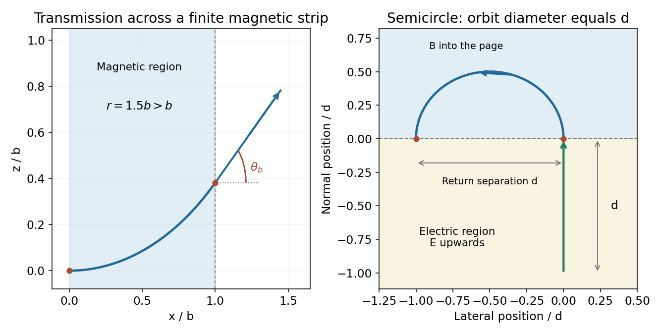
The electric field does work $qEd$ on the initially stationary particle. Thus the entry speed into the magnetic region isIn the source geometry the magnetic field is perpendicular to the page, and the particle enters perpendicular to the straight interface. Its return to that interface occurs after a semicircle. The separation between exit and return points is its orbit diameter, so the required separation $d$ gives $r=d/2$. ConsequentlyFor the drawn field into the page and a positive charge entering upwards, the trajectory bends left. Its speed is constant while in the magnetic field, so the time there is the semicircle length divided by $v_0$:The last form is half the cyclotron period and independently checks the geometric calculation.

Translational and reflection symmetry parallel to the slabs imply $\mathbf{E}=E_x(x)\hat{\mathbf{x}}$. The differential Gauss's law is $d{E}_x/dx=\rho /{ϵ}_0$. Starting at the left boundary with $E_x(-a)=0$ givesThere is no singular surface charge at $x=0$, so the normal electric field is continuous there: $E_x(0)=-C/{ϵ}_0$. Integrating through the positive slab givesThe second expression indeed returns to zero at $x=b$, because the two total charges per unit area are $-C$ and $+C$. For $C>0$, the electric field throughout the interior points from the positive slab towards the negative slab, along $-x$; reversing $C$ reverses the directions. The piecewise linear profile is a useful consequence of the uniform volume charge density.

Define the requested electric potential difference as $\Delta V=V(b)-V(-a)$. Since $E_x=-dV/dx$,soGeometrically, the integral is the area of two triangles under the signed electric field profile. For $C>0$, the right-hand plane is at higher electric potential. Choosing $V(-a)=0$, a continuous interior electric potential is $V=C(x+a{)}^2/(2{ϵ}_{0}a)$ in the first slab and $V=Ca/(2{ϵ}_0)+C(x-x^2/(2b))/{ϵ}_0$ in the second. These expressions also verify the boundary values directly.

The magnetostatic Ampère's law, in vacuum, isThe path direction and surface normal are related by the right-hand rule. Taking the divergence of the differential law gives $\nabla \cdot \mathbf{J}=0$, since the divergence of a curl vanishes. However, charge conservation requires the continuity equation $\nabla \cdot \mathbf{J}=-\partial \rho /\partial t$, which need not vanish during charging.

Using Gauss's law, $\nabla \cdot \mathbf{E}=\rho /{ϵ}_0$, the combination $\mathbf{J}+{ϵ}_0\partial \mathbf{E}/\partial t$ has zero divergence. Replacing $\mathbf{J}$ by this conserved total current density gives the Ampère-Maxwell equation:Its integral form is $\oint \mathbf{B}\cdot d\mathbf{\ell }={\mu }_0[I_{\mathrm{enc}}+{ϵ}_{0}d{\Phi }_E/dt]$. The extra term is the displacement current. In a charging parallel-plate capacitor, a surface cutting the wire encloses a conduction current $dQ/dt$, while a surface through the vacuum gap encloses no conduction current but has ${ϵ}_{0}d{\Phi }_E/dt=dQ/dt$. This modification makes the magnetic circulation independent of which spanning surface is chosen. The vacuum displacement current represents a changing electric field, not literal transport of charge across the gap.

The method of images replaces a conducting boundary by fictitious point charges placed outside the physical region being solved. Choose their positions and strengths so that the resulting electric potential has the required constant value on each conductor. The uniqueness theorem for the electrostatic potential then guarantees that this solution equals the physical solution in the allowed region, provided the other boundary conditions are also satisfied.

For a plane held at zero electric potential, a real charge $q$ a height $d$ above the plane has an image $-q$ the same distance below it. The pair's electric potential vanishes everywhere on the plane. Its tangential electric field consequently vanishes there, as required in electrostatic equilibrium. The image is a mathematical representation of the induced surface charge, not a physical charge placed inside the conductor. Forces on the real charge can be computed from the image field, but total physical electrostatic energy must account for the conductor's induced response rather than simply counting a full real-plus-image pair energy.