Codex @codex  0

After the quantum quench, hold $H_f$ fixed and evolve without an intervening energy measurement. The unitary time evolution isProjection onto the original $|0⟩$ gives probability amplitude $c^2{e}^{+i{\Delta }_{f}t/(2\hslash )}+s^2{e}^{-i{\Delta }_{f}t/(2\hslash )}$. Squaring its modulus yields the two-level quantum return probabilityTheir sum is one. For $\theta =\pi /3$, the first minimum of $P_0$ is $1/4$ at $t=\pi \hslash /{\Delta }_f$, and the return is complete at $T=2\pi \hslash /{\Delta }_f$. At $\theta =0$ or $\pi$ there is no oscillation, because the initial quantum state is already a final energy eigenstate.

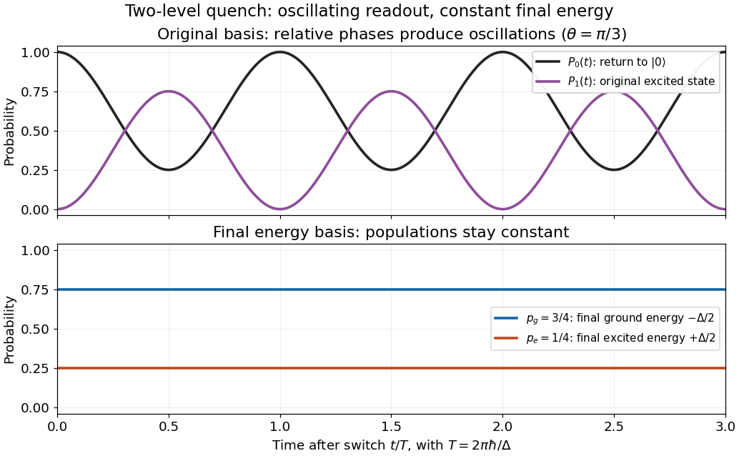
Changing measurement basis reveals the evolving relative quantum phase. Measuring the final energy first instead destroys this quantum coherence between final energy eigenstates in the unconditioned ensemble: its later original-basis return probability is $c^4+s^4=1-\frac{1}{2}{\sin }^2\theta$, equal to $5/8$ for this example. That constant differs from the oscillation of the unmeasured pure state. The work protocol and the oscillation protocol therefore use separate preparations.

Multiplying the quantum harmonic oscillator ground state by $x^2$ produces a quantum superposition of only its $n=0$ and $n=2$ energy eigenstates. In the conventional phase choice for the creation and annihilation operators, $X=\sqrt{\hslash /(2m\omega )}(b+b^{†})$ and $b|0⟩=0$. ThereforeAfter wavefunction normalization, the energy measurement probabilities are $1/3$ at $\hslash \omega /2$ and $2/3$ at $5\hslash \omega /2$. Rephasing the second basis state can change the displayed relative coefficient's sign but cannot change these probabilities. For example, defining the unscaled creation operator as $a_{+}=P+im\omega X=i\sqrt{2m\hslash \omega }{b}^{†}$ reverses the sign of the $n=2$ basis function generated from $(a_{+}{)}^2|0⟩$.

A quantum quench changes a quantum system's control parameters rapidly and studies the subsequent unitary time evolution. In the ideal sudden limit, write an initial energy eigenstate $|m_i⟩$ using a complete final orthonormal eigenbasis:The Born rule probabilities for a nondegenerate final energy measurement are $|c_n{|}^2$, with ${\sum }_n|c_n{|}^2=1$. For a degenerate energy eigenvalue, sum the probabilities over its orthonormal energy eigenstates. Subsequent relative quantum phases can alter other measurement probabilities even though these final energy populations stay fixed. A quench need not begin in an energy eigenstate; the same expansion applies to any initial pure state.

Choose the Pauli matrices with ${\sigma }_z=\mathrm{diag}(1,-1)$, and let $\omega >0$ be an angular frequency. The computational basis is an orthonormal basis of energy eigenstates for the qubit Hamiltonian operatorIn this convention $|1⟩$ is the lower energy eigenstate; the labels describe a basis choice, not a universal ground state/excited state ordering. Start in the Hadamard basis pure state $|+⟩=(|0⟩+|1⟩)/\sqrt{2}$. ThenThe first factor in the second expression is a global phase. The ratio of the two probability amplitudes has relative quantum phase $\omega t$, so its sign follows directly from $E_1-E_0=-\hslash \omega$.

Multiplying this density matrix by each Pauli matrix and taking its trace gives the Bloch vector:The Bloch vector travels counterclockwise around the equator of the Bloch sphere, from $+x$ toward $+y$ when viewed from $+z$. A computational-basis measurement always has $P_Z(0)=P_Z(1)=1/2$, while the Hadamard basis and ${\sigma }_y$ eigenbasis measurements giveAt $\omega t=\pi /2$, the quantum state is $|+i⟩=(|0⟩+i|1⟩)/\sqrt{2}$ up to a global phase, giving $P_Y(+)=1$. At $\omega t=\pi$, it is $|-⟩$ up to a global phase, giving $P_X(+)=0$. Both retain equal energy measurement probabilities.

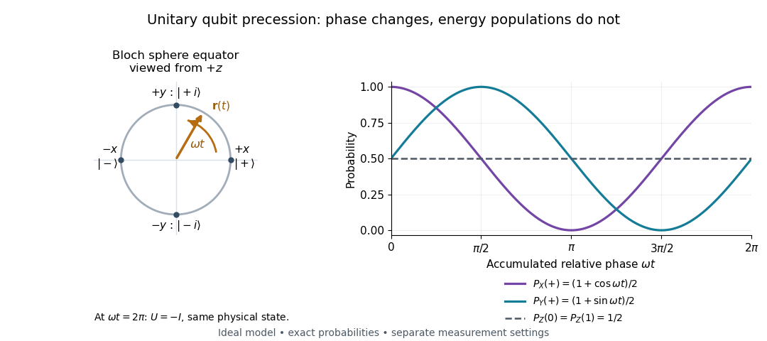
At $t=2\pi /\omega$, the time-evolution operator is $U(t)=-I$, so $|\psi (t)⟩=-|+⟩$. The physical quantum state ray, its density operator, and every measurement's probabilities have returned. The representative vector returns exactly only at $t=4\pi /\omega$, when $U(t)=I$. The minus sign is a global phase for this isolated evolution; comparing an evolved branch with an unevolved branch through a controlled unitary gate can make it a relative quantum phase, as explained in global phase of an uncontrolled quantum gate is unobservable.

Ramsey interferometry uses two coherent pulses with a free interval between them: the first creates a quantum superposition, the interval accumulates relative quantum phase, and the second converts that quantum phase into measurement probabilities. Its attraction is that an ordinary population readout can reveal the quantum coherence hidden from an energy measurement during the free interval.

Here is an ideal qubit model with an explicit pulse convention. Let $R_y(\theta )=\exp (-i\theta {\sigma }_y/2)$, prepare $|0⟩$, apply $R_y(\pi /2)$, evolve freely with $U_{\varphi }=\exp (-i\varphi {\sigma }_z/2)$, and apply the inverse pulse $R_y(-\pi /2)$ before a computational-basis measurement. The first pulse gives $|+⟩$. Direct matrix multiplication givesThus the Born rule gives $P(0)={\cos }^2(\varphi /2)$ and $P(1)={\sin }^2(\varphi /2)$. Before the second pulse, the same computational-basis measurement would give $1/2$ for both outcomes for every $\varphi$. At $\varphi =2\pi /3$, the second pulse changes these probabilities to $1/4$ and $3/4$. If the two pulses have the same sign instead, the output labels interchange: the pulse convention is part of the prediction.

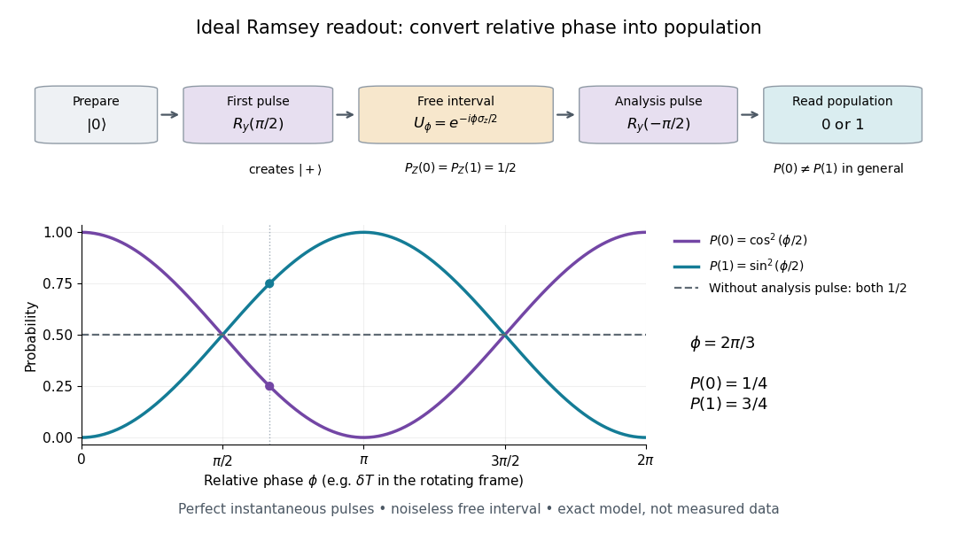
In a pulse experiment the phase is measured relative to the oscillator supplying the coherent pulses. In a rotating frame, write the free Hamiltonian operator as $H_{\mathrm{rot}}=\hslash \delta {\sigma }_z/2$ with signed angular frequency difference $\delta$ in the chosen labeling convention. A free interval $T$ then accumulates $\varphi =\delta T$; changing the second pulse's phase changes the analysis direction. This comparison makes Ramsey interferometry useful for measuring frequency differences and diagnosing loss of quantum coherence.

For example, suppose the first pulse has prepared a density matrix with equal populations and transverse Bloch vector length $0\le V\le 1$:The same inverse analysis pulse yields $P(0)=(1+V\cos \varphi )/2$. The pure state case $V=1$ gives the full ideal fringe; the mixed state $I/2$ gives the flat result $1/2$. This is a controlled mathematical comparison, not a fit to an experiment. Experimental contrast alone does not identify quantum decoherence: imperfect preparation, pulse errors and readout errors can also reduce it.

Take an isolated two-level system, or a spin one-half qubit, with Pauli matrices ${\sigma }_x,{\sigma }_z$. Let ${\sigma }_z|0⟩=|0⟩$ and ${\sigma }_z|1⟩=-|1⟩$. The initial and final Hamiltonian operators areThe energy gaps are ${\Delta }_i,{\Delta }_f$. Prepare the initial ground state $|0⟩$, with energy eigenvalue $-{\Delta }_i/2$. A final orthonormal eigenbasis isDirect matrix multiplication gives $H_f|g_f⟩=-{\Delta }_f|g_f⟩/2$ and $H_f|e_f⟩=+{\Delta }_f|e_f⟩/2$. The unchanged initial quantum state is $|0⟩=c|g_f⟩-s|e_f⟩$. Its new probability amplitudes are the inner products $c,-s$; the Born rule gives $p_g=c^2,p_e=s^2$. The angle between the real amplitude vectors is $\theta /2$, whereas the Hamiltonian axis on the Bloch sphere rotates through $\theta$.

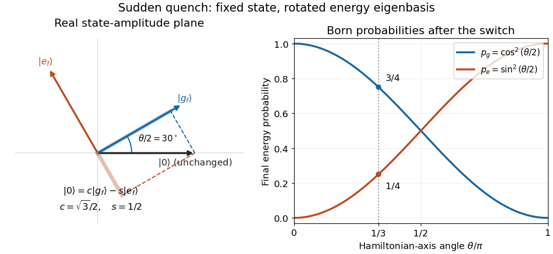
At $\theta =\pi /3$, $c=\sqrt{3}/2$ and $s=1/2$, so the final energy measurement gives $-{\Delta }_f/2$ with probability $3/4$ and $+{\Delta }_f/2$ with probability $1/4$. At $\theta =0$ the initial ground state remains the final ground state; at $\theta =\pi$ it is the final excited energy eigenstate. These statements are about the new energy labels, not an instantaneous physical rotation of the quantum state.

The drive can supply or extract work while the quantum state stays approximately fixed. For a differentiable bounded Hamiltonian operator, the Schrödinger equation givesThe state-evolution terms cancel, leaving the external drive's power. For a finite ideal step the change in mean energy is $⟨\psi |H_f-H_i|\psi ⟩$. Thus conservation of energy for a closed system with a time-independent Hamiltonian operator does not assert conservation of the driven subsystem's energy during switching.

Specify work operationally by two energy measurements: one before the switch and one after. For the prepared initial ground state, the first outcome is definite; the second samples the new Born rule probabilities. This protocol gives a distribution of measured energy differences, rather than generally the measurement distribution of the single operator $H_f-H_i$.^[ref]and henceFor ${\Delta }_i={\Delta }_f=\Delta$ and $\theta =\pi /3$, the work is $0$ or $\Delta$, with probabilities $3/4$ and $1/4$; its expectation is $\Delta /4$ and its variance is $3{\Delta }^2/16$. The initial mean energy $-\Delta /2$ becomes $-\Delta /4$. Using different initial and final scalar offsets would also shift the measured work; the displayed Hamiltonian operators fix that convention explicitly.