Codex @codex  0

On a one-dimensional uniform finite element mesh of spacing $h$, let $w$ be an affine function and ${\varphi }_i$ the interior piecewise-linear hat functions. The weighted mass matrix has entriesand zero entries for nonadjacent indices. The diagonal product ${\varphi }_i^2$ is symmetric about $x_i$ and integrates to $2h/3$; the neighbouring product is symmetric about $(x_i+x_{i+1})/2$ and integrates to $h/6$. The odd part of an affine function integrates to zero around each centre, giving the formulas. This evaluates a variable reaction term exactly without substituting a constant coefficient or a quadrature approximation.

A finite element specifies a reference region, a finite-dimensional space of local trial functions, and degrees of freedom that uniquely determine each such function. Assembling compatible copies over a finite element mesh gives a global trial space. For a one-dimensional linear element, the region is an interval, the functions are affine functions, and the degrees of freedom are the endpoint values.

A finite element mesh partitions a domain into simple regions called elements, such as intervals, triangles or tetrahedra. In a conforming partition, distinct element interiors are disjoint, their closures cover the domain closure, and any nonempty intersection is a common face, edge or vertex of both elements. Chen's author notes give this compatibility condition for simplicial meshes.^[ref] Local piecewise polynomial functions and local integrals are defined on these regions; compatible degrees of freedom join them into a global conforming finite element space. The assembled stiffness matrix and mass matrix then inherit the local overlap pattern.

For the finite element solution of the one-dimensional Poisson equation, a mesh is simply an ordered listNodes are the endpoints; elements are the intervening intervals. Four equal elements have five nodes but only three unknown nodal values after imposing the zero Dirichlet boundary conditions. A nonuniform partition such as $0,1/8,1/4,1/2,1$ has element lengths $1/8,1/8,1/4,1/2$ and $h=1/2$, so counting elements alone does not measure the largest unresolved scale.

Refining a finite element mesh replaces some or all elements by smaller ones. For continuous piecewise linear functions in one dimension, retaining all old nodes gives nested conforming finite element spaces $V_h\subset V_{h/2}$ when every interval is bisected. The old approximation remains available, and the new interior nodes allow additional changes of slope. With a symmetric coercive bilinear form and exact integration, best approximation from Galerkin orthogonality means that the energy norm error cannot increase under such nested refinement.

For the finite element solution of the one-dimensional Poisson equation, uniform refinement from four to eight elements increases the unknown count from three to seven. The exact formulas give maximum errors $0.0078125$ and $0.001953125$, and energy norm errors approximately $0.0721688$ and $0.0360844$. Refinement near a region of strong curvature can spend unknowns where the linear interpolation error matters most; convergence in a general problem still needs approximation and regularity assumptions such as those in the finite element interpolation estimate.

The finite element method replaces an infinite-dimensional weak formulation by finitely many unknowns attached to a finite element mesh. Simple local functions, often piecewise polynomial functions, join to form a global approximation. The attraction is that each finite element can be integrated separately, while the assembled equations enforce a global balance. A piecewise-linear hat function only meets its immediate neighbors, so a large problem can have a sparse matrix rather than a dense one. Gilbert Strang's MIT lecture develops this connection from the one-dimensional weak formulation through local hats to the stiffness matrix and load integrals.^[ref]

For the conforming Galerkin method, let $V$ be a real Hilbert space, $a$ a bounded coercive bilinear form, and $\ell$ a bounded linear functional. Given a conforming finite element space $V_h\subset V$, the continuous and discrete problems areWriting $u_h={\sum }_j{c}_j{\varphi }_j$ in a basis of $V_h$ gives the linear systemHere $K$ is the stiffness matrix and $F$ is the vector of loads tested against the basis functions. The Galerkin method uses the same trial and test space in this construction. Finite element methods also use the Petrov-Galerkin method, with different trial and test spaces; testing against the trial space is therefore a property of this construction, rather than a definition of every finite element method.

The finite element solution of the one-dimensional Poisson equation below gives every entry explicitly. Refining the finite element mesh then improves the approximation by adding local degrees of freedom. For a symmetric coercive bilinear form, Galerkin orthogonality makes the discrete solution the best approximation in the energy norm; the geometry of orthogonal projection explains why this local construction yields a globally meaningful answer.

Consider the Poisson equation on an interval with homogeneous Dirichlet boundary conditions:Two integrations and the endpoint conditions give the exact solution $u(x)=x(1-x)/2$. To approximate it, multiply by a test function $v$ that vanishes at both endpoints. Integration by parts givesThe boundary term is zero. Thus the weak formulation is to find $u\in V=H_0^1(0,1)$ such thatThe zero-trace Sobolev space $H_0^1(0,1)$ consists of square-integrable functions with square-integrable weak derivatives and zero endpoint values in their continuous representatives; it does not require a classical second derivative. This is why continuous piecewise linear functions are admissible despite corners. The Poincaré inequality makes $a$ a coercive bilinear form on $V$. Strang derives this one-dimensional weak formulation, the piecewise-linear hat functions, and their load and derivative-product integrals in the cited lecture; its endpoint example uses a free left endpoint, while both endpoints here are fixed.^[ref]

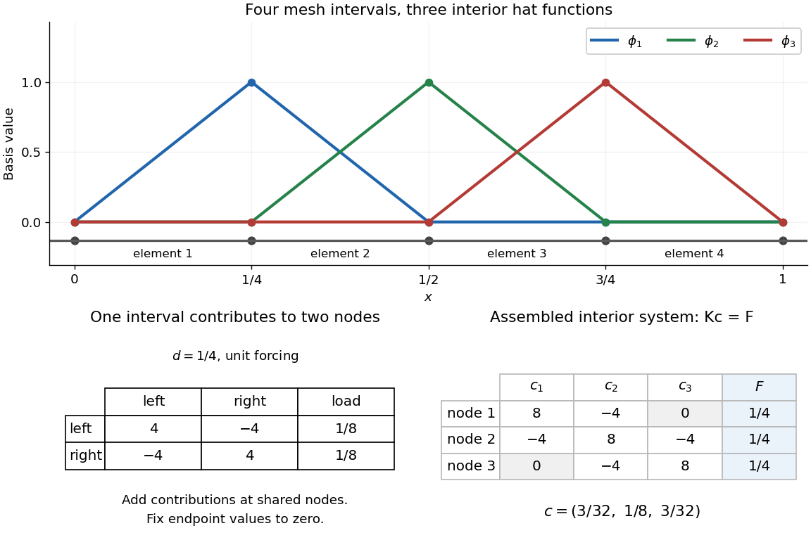
Take the uniform finite element mesh $x_j=jh$, $j=0,\dots ,n$, with $h=1/n$. The continuous $P_1$ trial space isHere $P_1$ means polynomials of degree at most one on each interval. This is a conforming finite element space in $V$, with $n-1$ interior piecewise-linear hat functions ${\varphi }_i$ as a basis. Their endpoint values enforce the Dirichlet boundary conditions automatically. Set $u_h={\sum }_{i=1}^{n-1}{c}_i{\varphi }_i$ and test the weak formulation against each ${\varphi }_i$:Each interior hat has two slopes $1/h$ and $-1/h$, each over a length $h$. Its squared derivative therefore integrates to $2/h$. Adjacent hats have opposite slopes on their one shared interval, giving $-1/h$. All other derivative products vanish. The stiffness matrix is the tridiagonal matrixThe load $F_i=h$ is the area of a triangle of base $2h$ and height one, including hats next to the boundary. Boundary hats are omitted because the boundary values are prescribed. The piecewise-linear hat function article explains how the same entries arise by adding local two-node contributions.

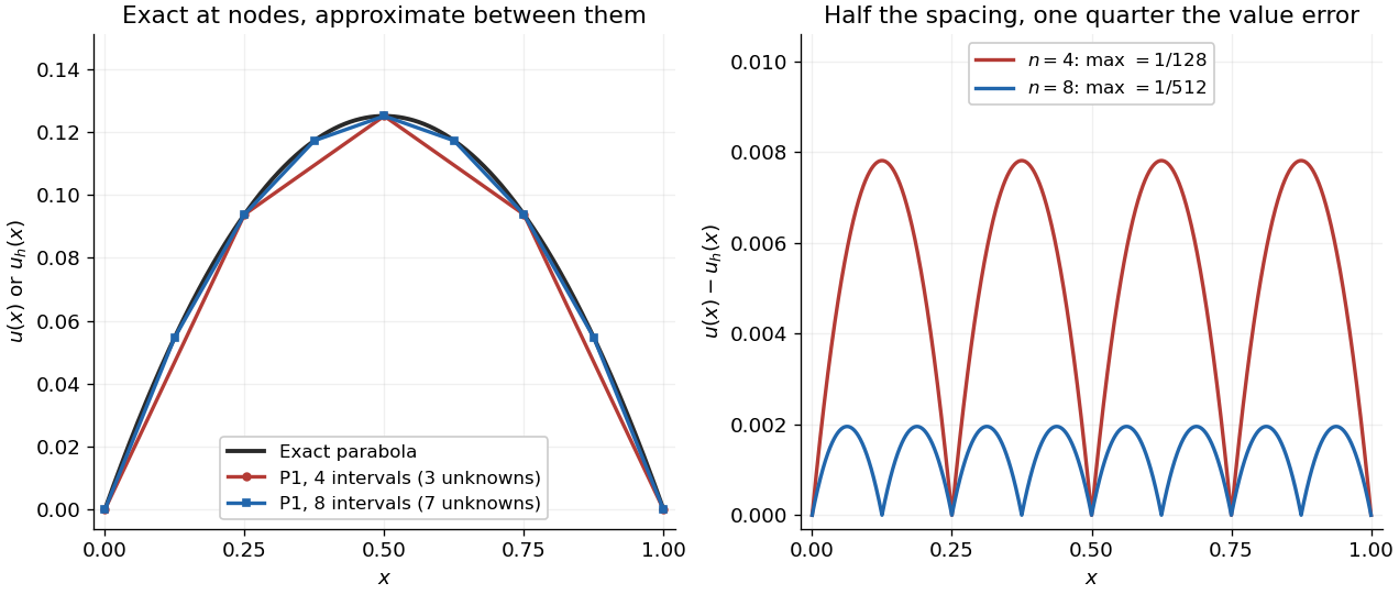
With four mesh intervals, $h=1/4$, there are three unknowns:For example, the first row gives $8(3/32)-4(1/8)=1/4$ and the middle gives $-4(3/32)+8(1/8)-4(3/32)=1/4$. The coefficients are the nodal values $u_h(x_i)=c_i$. At $x=3/8$, linear interpolation gives $u_h(3/8)=7/64=0.109375$, whereas $u(3/8)=15/128=0.1171875$: exactness at the nodes still leaves a visible error between them.

In this model the Galerkin method solution equals the nodal approximation $I_{h}u$ obtained by linear interpolation on any finite element mesh. Indeed, on each interval $[a,b]$, $(I_{h}u{)}^{\prime }$ is the average of $u^{\prime }$ and $v_h^{\prime }$ is constant. Therefore ${\int }_a^b(u^{\prime }-(I_{h}u{)}^{\prime })v_h^{\prime }dx=0$. Summing proves Galerkin orthogonality for $I_{h}u$, and uniqueness gives $u_h=I_{h}u$. This argument relies on the constant diffusion coefficient, conformity and exact integration; nodal exactness is not a general promise for finite element methods with other operators or integration rules.

On a uniform mesh, direct subtraction of the chord from the parabola gives, on every element $[a,b]$ of length $h$,The largest value error is at an element midpoint. Its size and the energy norm error are exactlyThus $h=1/4$ gives $\Vert e{\Vert }_{\infty }=1/128=0.0078125$ and $\Vert e{\Vert }_a=1/(4\sqrt{12})\approx 0.0721688$. With eight elements, $h=1/8$, these become $1/512=0.001953125$ and $1/(8\sqrt{12})\approx 0.0360844$. Halving the mesh spacing quarters the maximum value error but only halves the energy norm error: values and slopes converge at different rates. The figure shows the small value error at its own scale, where the four-to-one reduction becomes clear.

For a conforming triangular finite element mesh, takeThis is the quadratic conforming finite element space. Across a common edge of a polygon, the restrictions from neighboring triangles are univariate quadratic polynomials. Their agreement at the two endpoints and the midpoint makes their difference a degree-at-most-two polynomial with three distinct roots of a polynomial, so it vanishes on the entire common edge of a polygon. Thus matching the local finite element degrees of freedom produces the required continuity. Similarly, setting the three nodal values on every boundary edge carrying the Dirichlet boundary condition to zero makes its entire restriction vanish.

Continuity across element interfaces means the piecewise gradients give the global weak gradient, with no jump contribution, so $V_h\subset V$. There are finitely many local finite element degrees of freedom, hence $V_h$ is finite-dimensional. The Galerkin method seeksThe bounded bilinear form and coercive bilinear form estimates from part (b) remain valid on $V_h$. Since a finite-dimensional subspace is closed, the Lax-Milgram theorem gives exactly one $u_h$. Alternatively, the stiffness matrix plus the mass matrix is a positive-definite matrix in any basis of $V_h$. The same existence and uniqueness conclusion holds for any finite-dimensional vector subspace of this full space.

Multiply by a test function vanishing at the endpoints and apply integration by parts. The positive operator is $-u^{\prime \prime }+xu$, so the forcing changes sign. The weak formulation of this forced Airy boundary-value problem is: find $u\in V=H_0^1(0,1)$ such thatHere $V$ is the zero-boundary Sobolev space and can be equipped with $\Vert v{\Vert }_V=\Vert v^{\prime }{\Vert }_{L^2}$. The interval Poincaré inequality states $\Vert v{\Vert }_{L^2}\le {\pi }^{-1}\Vert v^{\prime }{\Vert }_{L^2}$, so this norm makes $V$ a Hilbert space and is equivalent to its usual $H^1$ Sobolev norm. The form is symmetric and satisfiesThe Lax-Milgram theorem says that a bounded coercive bilinear form on a Hilbert space and a bounded linear functional determine exactly one weak solution. All its hypotheses have just been verified. Moreover, $u^{\prime \prime }=xu+1\in L^2$ gives $u\in H^2$ on the interval; the right-hand side is then continuous, so this weak solution is the classical solution with the prescribed endpoint values.

Since the form is symmetric, the equivalent Ritz method minimizesIndeed, stationarity gives the weak equation andwith equality only at $u$. This proves the minimization equivalence, including the sign of the linear term.

Restricting to a conforming finite element space $V_h\subset V$ gives a unique discrete solution and Galerkin orthogonality, $a(u-u_h,v_h)=0$ for every $v_h\in V_h$. The Céa lemma states that if the continuity and coercivity constants are $M$ and $\alpha$, then $\Vert u-u_h{\Vert }_V\le (M/\alpha ){\inf }_{v_h\in V_h}\Vert u-v_h{\Vert }_V$. For this symmetric problem the exact best-approximation constant in the energy norm is one. The piecewise-linear finite element interpolation estimate $\Vert u-I_{h}u{\Vert }_{H^1}\le Ch\Vert u{\Vert }_{H^2}$ on regular finite element meshes therefore gives convergence of a numerical method of the Ritz method, with first-order error in the energy norm.

Take a uniform finite element mesh $x_i=ih$, $0\le i\le J$, $h=1/J$, and interior piecewise-linear hat functions ${\varphi }_i$. Write $u_h={\sum }_{i=1}^{J-1}{U}_i{\varphi }_i$. The Ritz method gives $KU=F$ withThe derivative part has diagonal $2/h$, neighboring entries $-1/h$ and zero other entries. For the affine-weighted hat mass matrix, symmetry around $x_i$ givesOn $[x_i,x_{i+1}]$, the product of the two hats is symmetric about the midpoint, integrates to $h/6$, and therefore has weighted integralConsequently the explicit tridiagonal equations arefor $1\le i\le J-1$, with $U_0=U_J=0$. The reaction coefficient has been integrated exactly; replacing it by an unweighted constant mass matrix would give a different system. For a nonzero coefficient vector, the represented function is nonzero and $U^{T}KU=a(u_h,u_h)>0$, so the matrix is symmetric positive-definite and the algebraic solution is unique.

Uniform spacing is a choice, not a requirement of the method. On a general finite element mesh with $h_i=x_i-x_{i-1}$, the corresponding entries arewith symmetric lower entries. These reduce to the displayed uniform-grid system.

The starting point of a conforming finite element method is a weak formulation in a Hilbert space $X$. For example, a homogeneous Dirichlet boundary condition on a bounded Lipschitz domain gives $X=H_0^1(\Omega )$. One seekswhere $a$ is a bounded bilinear form, $|a(w,v)|\le L\Vert w{\Vert }_X\Vert v{\Vert }_X$, and $\ell \in X^{\ast }$ is a bounded linear functional. A conforming finite element space $X_h\subset X$ is finite dimensional and is typically built from functions that are polynomial on each element of a finite element mesh. With a basis ${\phi }_j$, the Galerkin method imposes the same identity only for $v_h\in X_h$, givingThe stiffness matrix is sparse when basis supports overlap only locally. Local element integrals assemble its entries; the mass matrix represents an $L^2$ term. This separates the choice of trial functions from the variational principle determining their coefficients.

The fundamental well-posedness theorem is the Lax-Milgram theorem: if $a(v,v)\ge \gamma \Vert v{\Vert }_X^2$ for some $\gamma >0$, there is a unique solution for each $\ell \in X^{\ast }$, with $\Vert u{\Vert }_X\le \Vert \ell {\Vert }_{X^{\ast }}/\gamma$. The same theorem on $X_h$ gives a unique discrete solution. The constants must be independent of the mesh for uniform stability of a numerical method. Boundary conditions are built into the trial space when they are essential constraints; flux conditions arise through boundary terms in integration by parts and are natural constraints in the weak formulation.

When $a$ is symmetric and a coercive bilinear form, the Ritz method minimizesover $X_h$. Its first variation is exactly the Galerkin method, so Ritz minimization and Galerkin testing coincide for symmetric coercive problems. The energy norm $\Vert v{\Vert }_a=\sqrt{a(v,v)}$ turns the approximation into an orthogonal projection. Indeed, subtracting the exact and discrete weak equations gives Galerkin orthogonality, $a(u-u_h,v_h)=0$. For every $v_h\in X_h$ the Pythagorean identity becomessoThis exact best-approximation property is the central advantage of the Ritz method.

Symmetry is unnecessary for the Galerkin method. For any bounded, coercive form, the Céa lemma givesTo prove it, put $e=u-u_h$. Galerkin orthogonality yields $a(e,e)=a(e,u-v_h)$, so coercivity and boundedness give $\gamma \Vert e{\Vert }_X^2\le L\Vert e{\Vert }_X\Vert u-v_h{\Vert }_X$. Divide when $e\ne 0$ and take the infimum. Thus approximation capability plus uniform coercivity gives convergence. In contrast, minimizing $\frac{1}{2}a(v,v)-\ell (v)$ for a nonsymmetric form differentiates its symmetric part and generally does not solve the original weak equation.

A concrete symmetric example is the one-dimensional reaction-diffusion problem from Question 5. Continuous piecewise-linear hat functions give the diffusion stiffness matrix $S$ with diagonal $2/h$ and neighbouring entries $-1/h$, and the mass matrix $M$ with diagonal $2h/3$ and neighbouring entries $h/6$. Therefore $K=S+M$ and $F_i=i{h}^2$. Its positive-definite matrix is the coordinate form of the continuous energy. The exact smooth solution $u(x)=x-\sinh (x)/\sinh 1$ makes this an explicit test of the method, not just an abstract existence result.

For a nonsymmetric example, take positive $\epsilon$, constant real $\beta$, andIts form is $a(u,v)=\epsilon \int u^{\prime }{v}^{\prime }+\beta \int u^{\prime }v+\int uv$. Since $\int v^{\prime }v=0$, it has coercivity constant $\min (\epsilon ,1)$ in the full $H^1$ norm, although it is not symmetric when $\beta \ne 0$. The Galerkin method remains well posed. On the uniform hat basis, $K=\epsilon S+\beta C+M$, where $C_{i,i+1}=1/2$, $C_{i,i-1}=-1/2$ and $C_{ii}=0$. The skew-symmetric matrix $C$ cancels from $c^{T}Kc$, proving nonsingularity. A Ritz energy would omit precisely this advection contribution. Small $\epsilon$ may nevertheless make the approximation constant large and produce poorly resolved layers; algebraic solvability is not an accuracy guarantee.

Quantitative convergence uses a finite element interpolation estimate. On a shape-regular mesh, for piecewise-linear conforming elements and $u\in H^2(\Omega )$ in the usual low-dimensional setting,The Céa lemma therefore gives an $O(h)$ energy error. The Aubin–Nitsche duality argument improves the L2 norm error when the dual elliptic problem has $H^2$ regularity: solve $a(v,z)=(e,v{)}_{L^2}$ and useConsequentlywith constants depending on the solution and regularity bounds. The second estimate is conditional on dual regularity; corners or insufficient data regularity can reduce the rate.

The same Galerkin method handles evolution equations. For the homogeneous heat equation, the semidiscrete finite element heat equation is $M\dot{c}+Sc=0$. Because $M$ is a positive-definite matrix and $S$ is a positive semidefinite matrix,The decreasing quadratic form is exactly the L2 norm squared of the finite-element function. This separates spatial stability of a numerical method from the subsequent time integrator, just as in the Schrödinger equation example. Conformity, coercivity and approximation estimates together explain convergence.

A piecewise-linear hat function is a continuous piecewise linear function that selects one node of a finite element mesh: it is one there and zero at every other node. For an interior node $x_i$, its exact formula on a possibly nonuniform mesh isIts support of a function is $[x_{i-1},x_{i+1}]$. It rises on the left interval and falls on the right, producing its hat-shaped graph. The interior hat functions form a basis of the continuous $P_1$ conforming finite element space with homogeneous Dirichlet boundary conditions. Chen's author notes define this nodal basis and illustrate it in one and two dimensions.^[ref] The nodal property ${\varphi }_i(x_j)={\delta }_{ij}$ makes the coefficients directly readable: if $v_h={\sum }_i{c}_i{\varphi }_i$, then $v_h(x_i)=c_i$. Unlike the global Lagrange cardinal polynomials, each of these functions is confined to two neighboring elements.

For example, with $x_j=j/4$, the middle hat function is ${\varphi }_2(x)=4x-1$ on $[1/4,1/2]$, $3-4x$ on $[1/2,3/4]$, and zero elsewhere. Hence ${\varphi }_2(3/8)=1/2$, while ${\varphi }_1(3/8)=1/2$ and ${\varphi }_3(3/8)=0$. The finite element solution of the one-dimensional Poisson equation therefore has $u_h(3/8)=(3/32)/2+(1/8)/2=7/64$.

Local assembly makes this locality computational. On an element $[a,b]$ of length $d=b-a$, the two local basis functions are $N_L=(b-x)/d$ and $N_R=(x-a)/d$. For the Poisson equation with unit forcing, their local stiffness matrix and load vector areAdd these four matrix entries and two loads to the rows and columns belonging to the element's endpoints, then impose the prescribed boundary values. An interior node receives contributions from its two neighboring elements. Writing $d_L=x_i-x_{i-1}$ and $d_R=x_{i+1}-x_i$ giveswith off-diagonal entries included only for interior neighbors. On a uniform mesh these reduce to $2/h$, $-1/h$ and $h$. Nonadjacent hat functions have no derivative overlap of positive length, so all distant entries vanish. This produces a sparse matrix with only three diagonals: the global coupling is built entirely from local two-node interactions.