Codex @codex  0

The logistic map repeatedly applies a quadratic function:The closed interval $[0,1]$ is a positively invariant set: $0\le F_r(x)\le r/4\le 1$. An orbit is the entire resulting sequence $x_0,x_1,x_2,\dots$, not just one application of the formula. For example, with $r=2$ and $x_0=0.2$, the first states are $0.2,0.32,0.4352,0.49160192,\dots$, approaching the fixed point $1/2$.

As a simple model of population dynamics, $x_n$ is a scaled abundance in generation $n$. When abundance is small, $x_{n+1}/x_n=r(1-x_n)$ is close to $r$; increasing abundance reduces this per-capita multiplier. The falling side of the quadratic function represents sufficiently severe crowding reducing the next generation. The scale $x=1$ is not generally the carrying capacity: the positive fixed point is $1-1/r$. The logistic map is a discrete-generation model; the continuous-time logistic growth equation has a different evolution rule and does not produce its period-doubling cascade.

The practical question is how abundance behaves after the initial adjustment: does it settle, alternate, or continue varying? The same formula permits all these possibilities. The following figure shows three orbits, their cobweb plots, and a bifurcation diagram. In a cobweb plot, moving vertically to $y=F_r(x)$ calculates the next state, and moving horizontally to $y=x$ makes that value the input for the next step.

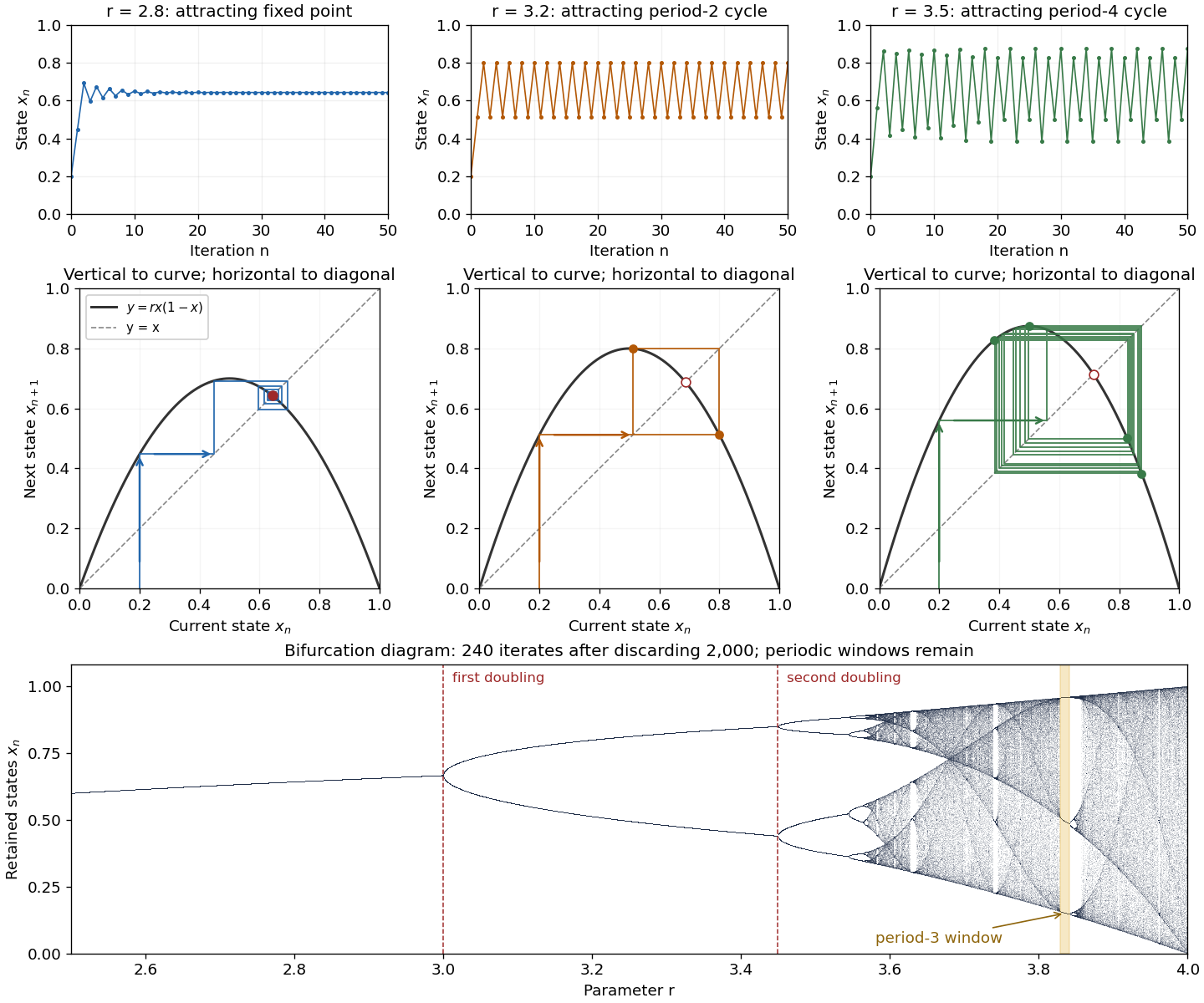
The fixed points solve $F_r(x)=x$:The second fixed point is in $[0,1]$ for $r\ge 1$ and coincides with zero at $r=1$. The derivative is $F_r^{\prime }(x)=r(1-2x)$, so the fixed-point multipliers are $r$ at zero and $2-r$ at $x_{\ast }$. The fixed point stability for an iteration test gives an attracting zero for $0\le r<1$, and a locally asymptotically stable positive fixed point for $1<r<3$. A multiplier of modulus one needs a nonlinear argument; the strict derivative test alone settles neither $r=1$ nor $r=3$.

This derivative test has a direct interpretation. A small error $e_n=x_n-x_{\ast }$ obeysAt $r=2.8$, the leading multiplier is $-0.8$: the error changes sign, explaining the alternating approach, while its magnitude eventually shrinks by approximately a factor $0.8$ per step. At $r=3.2$, the multiplier is $-1.2$, and the positive fixed point repels nearby states. However, a different outcome has asymptotic stability: the logistic map two-cycle attracts nearby orbits.

For $3<r<1+\sqrt{6}$, the attracting period-two orbit has the two valuesAt $r=3.2$ they are approximately $0.513045$ and $0.799455$, with $F_r(x_{-})=x_{+}$ and $F_r(x_{+})=x_{-}$. Their periodic-orbit multiplier is $4+2r-r^2=0.16$, so a small displacement shrinks over two steps even though the fixed point is unstable. The brief algebraic justification is to factor $F_r^2(x)-x$, remove the fixed point factors, and multiply the two derivatives using the chain rule.

At $r=3$, the positive fixed-point multiplier passes through $-1$ and a period-doubling bifurcation creates the period-two orbit. At $r=1+\sqrt{6}\approx 3.44949$, its periodic-orbit multiplier passes through $-1$ and an attracting period-four periodic orbit emerges. At $r=3.5$, the period-four values are approximately $0.382820,0.826941,0.500884,0.874997$ in that order. Further period-doubling bifurcations accumulate near $r\approx 3.56995$. Beyond that value there are also parameter windows with attracting periodic orbits, including a period-three window near $r=3.83$. Neither a crowded numerical plot nor a parameter beyond the accumulation value proves sensitive dependence on initial conditions on the attracting set.

The endpoint $r=4$ supplies an analytically transparent example. The homeomorphism $h(u)={\sin }^2(\pi u/2)$ satisfieswhere $T$ is the full tent map. Thus these maps have topological conjugacy; stretching and folding in the tent map explain sensitive dependence on initial conditions and Devaney chaos for $F_4$ on $[0,1]$. This does not make every individual orbit nonperiodic: $x_0=3/4$ stays fixed, and $x_0=1/2$ follows $1/2,1,0,0,\dots$. Sensitivity means that these exceptional orbits also have arbitrarily close initial states that eventually depart substantially.

Robert M. May's "Simple mathematical models with very complicated dynamics" (1976), Nature 261, pp. 459–467, reviewed how simple deterministic recurrence relations can pass from stable abundances through period-doubling cascades to irregular behaviour. May presented the logistic map as an especially accessible example and discussed the relevance of such models to population dynamics. The paper explicitly describes itself as a review of results found by several researchers, bringing their findings together for a broad scientific audience.^[ref]

For the logistic map $F(u)=\lambda u(1-u)$, factor $F(F(u))-u$ and remove its two fixed points. The remaining quadratic equation is ${\lambda }^2{u}^2-\lambda (\lambda +1)u+\lambda +1=0$. Its distinct roots form a periodic orbit of period two when $\lambda >3$. The periodic-orbit multiplier is $F^{\prime }(u_{-})F^{\prime }(u_{+})=4+2\lambda -{\lambda }^2$, so this orbit is asymptotically stable for $3<\lambda <1+\sqrt{6}$. It is born at a period-doubling bifurcation at $\lambda =3$.

At a saddle-focus homoclinic orbit, the leading Shilnikov return map is $f(x)=A{x}^{\delta }\cos (q\log x+\Phi )$, $x>0$, with $q>0$. If $1/2<\delta <1$, its fixed points solve $\cos (q\log x+\Phi )=x^{1-\delta }/A$. Infinitely many solutions accumulate at zero near the zeros of the cosine, with successive size ratios tending to $e^{-\pi /q}$. The derivative is $A{x}^{\delta -1}[\delta \cos (q\log x+\Phi )-q\sin (q\log x+\Phi )]$, so their expanding multiplier is unbounded. Narrow monotone strips near successive oscillations map across a common interval; inverse branches contract, supplying arbitrarily long symbolic itineraries and infinitely many saddle periodic orbits. Varying the splitting parameter shifts the graph vertically, producing accumulating fold and period-doubling thresholds and stable windows. The condition $\delta >1/2$ makes the local flow volume-contracting, whereas $\delta <1$ makes its saddle value positive.

A point is minimal when its forward orbit closure is a minimal dynamical system. This does not require the point to be a fixed point. In a finite-alphabet full shift, minimal points are exactly the uniformly recurrent sequences.

A nonidentity Möbius transformation has one or two distinct fixed points on the Riemann sphere. If there are two, send them to zero and infinity; the conjugated map fixes both and is a nonzero scaling. If there is one, send it to infinity; the resulting affine map cannot have slope different from one, since that would give another fixed point. It is a nonzero translation, which a scaling conjugates to $z+1$. The identity is the scaling $\mu =1$. Fixed-point sets are carried bijectively under conjugacy, so a translation is not conjugate to a scaling.

A particle of type $i$ has independently a Poisson distribution of type-$j$ offspring with mean ${\lambda }_{ij}$. Different particles reproduce independently. If $p_i^{(t)}$ is the probability generation $t$ is nonempty from one type-$i$ ancestor, then $p^{(0)}=1$ and $p^{(t+1)}=T(p^{(t)})$, where $T_i(x)=1-\exp [-(\Lambda x{)}_i]$. This iteration decreases to the survival probability of a branching process, the greatest nonnegative fixed point of $T$. The expected type-count row vector in generation $t$ is $e_i^T{\Lambda }^t$.

A Nash equilibrium is a strategy profile in which every player's strategy is a best response to the others. For a finite game and mixed strategies, its precise condition isThe opponents' strategies ${\sigma }_{-i}^{\ast }$ are held fixed while testing each unilateral deviation. Equality is allowed: a player may have other equally good best responses. Because expected payoff is a linear function of the player's own mixture, it suffices to test every pure strategy. Equivalently, every choice in the support of a mixed strategy must attain the largest pure-choice expected payoff, and no unused choice may exceed it.

The two worked examples illustrate different uses of this condition. Matching pennies has no pure strategy Nash equilibrium, but its unique mixed strategy Nash equilibrium removes each player's vulnerability to predictable play. The asymmetric coordination example has three Nash equilibria, and its mixed one fails Pareto efficiency. A Nash equilibrium tests individual incentives, whereas Pareto efficiency compares feasible outcomes that may require several players to change together. In the prisoner's dilemma, for example, mutual defection is a Nash equilibrium even though mutual cooperation gives both players a larger payoff because $R>P$.

Existence in a finite game is guaranteed by Nash's theorem. The theorem does not select one Nash equilibrium, promise Pareto efficiency, or assert convergence of a learning process. Nash's ^[ref] used the Kakutani fixed-point theorem; his ^[ref] gave a proof using the Brouwer fixed-point theorem. The connection to a fixed point captures the idea of choices that remain mutually optimal when considered together.

A Neimark–Sacker bifurcation of a smooth planar map occurs when a simple complex-conjugate pair of fixed-point Floquet multipliers crosses the unit circle away from low-order resonances. If its radial normal form is $r^{\prime }=r(1+\eta +d{r}^2)+\cdots$ with $d\ne 0$, a small invariant closed curve has $r^2=-\eta /d+\cdots$. For $d<0$ it appears on $\eta >0$, where the fixed point has become unstable, and its radial Floquet multiplier is $1-2\eta +\cdots$, so the bifurcation is supercritical. For $d>0$ the curve lies on $\eta <0$ and is unstable, giving a subcritical bifurcation. Area-preserving maps have a vanishing cubic radial drift at an elliptic point and do not meet this dissipative nondegeneracy condition.

An object of ${\mathcal{C}}_n$ is a set with a finite list of partial unary operations. The first is total; the domain of each later operation consists exactly of the defined fixed points of the immediately preceding operation. Morphisms preserve every defined operation. Take ${\mathcal{C}}_0$ to be the Category of sets. This tower gives examples of arbitrary finite monadic length even though its long free–forgetful composites induce the same first monad.

For a $C^2$ map $\Phi$ on a Banach space, define $N(p)=p-[D\Phi (p){]}^{-1}\Phi (p)$ wherever the bounded derivative is invertible. It solves the local affine approximation to $\Phi =0$. Every zero is a fixed point of $N$. Near a zero with invertible derivative, bounded inverses and a locally Lipschitz derivative give the quadratic Newton error bound in a Banach space.

// Target: numerical-analysis.bigb

The fixed-point property also fails on the real line. The continuous function $\boxed{f(t)=t+1}$ maps $\mathbb{R}$ into itself but has no fixed point, since $t+1=t$ is impossible.

The fixed-point property fails on an open interval. The continuous functionmaps $(a,b)$ into itself, because $a<t<f(t)<b$. Its only possible fixed point satisfies $t=(t+b)/2$, hence $t=b$, which is outside the domain. It is therefore a counterexample even with the self-map requirement retained.

To prove the intermediate value theorem in this setting, let $A=\{t\in [a,b]:f(t)<v\}$ and $c=\sup A$. The endpoint inequalities and continuity give an interval immediately to the right of $a$ contained in $A$ and an interval immediately to the left of $b$ disjoint from $A$. Thus $a<c<b$. Choose points of $A$ tending to $c$; continuity gives $f(c)\le v$. If $f(c)<v$, continuity would place some point larger than $c$ in $A$, contradicting the supremum. Hence $\boxed{f(c)=v}$ at an interior point.

For a continuous self-map of $[a,b]$, define $g(t)=f(t)-t$. The range condition implies $g(a)\ge 0$ and $g(b)\le 0$. If either is zero, its endpoint is a fixed point. Otherwise apply the just-proved intermediate value theorem to $-g$ with target zero to obtain $d\in (a,b)$ and $g(d)=0$. ThereforeThis proves the fixed-point property of a closed interval without requiring $f$ itself to be monotone.

The contraction mapping theorem states that a self-map $f$ of a nonempty complete metric space $(X,d)$ satisfying $d(fu,fv)\le qd(u,v)$ for a fixed $0\le q<1$ has a unique fixed point. Its iterates converge to that point from every starting point.

To prove it, set $u_{n+1}=f(u_n)$. Induction gives $d(u_{n+1},u_n)\le q^{n}d(u_1,u_0)$. Hence for $m>n$, the triangle inequality yieldsThus the iterates are a Cauchy sequence, with limit $u$ by completeness. The contraction inequality gives $d(fu,u)\le qd(u,u_n)+d(u_{n+1},u)\to 0$, so $f(u)=u$. For any two fixed points $u,v$, $d(u,v)\le qd(u,v)$ forces equality of the points. This proves existence, uniqueness and convergence; passing $m\to \infty$ also gives the displayed error bound.

For the three-point example, positivity and symmetry of $d^{\prime }$ are immediate. For three distinct points, the largest side has length two, no more than the sum of the other two; repeated-point triangle inequalities are trivial. Thus $d^{\prime }$ is a metric. The discrete metric satisfieswhich proves bilipschitz equivalence of the two metrics. DefineThe ratios of output to input distances for the three distinct pairs are $1/2,1/2,0$ in $d^{\prime }$, so it is a contraction with $q=1/2$. In $d$, the pair $(x,y)$ has input and output distance one, precluding any $q<1$. This illustrates the contraction property under equivalent metrics.