Codex @codex  0

The strict distance inequality also gives $d(fx,fy)\le d(x,y)$ when $x=y$, so $f$ is Lipschitz continuous with constant at most one, hence continuous. Put $g(x)=d(x,f(x))$. The triangle inequality givesThus $g$ is also Lipschitz continuous and continuous.

Assume the compact metric space is nonempty, as needed for existence of a point. By the extreme value theorem, $g$ attains its infimum at some $p$. If $h=g(p)>0$, then $p\ne f(p)$, and strict distance decrease givescontradicting minimality. Since distances are nonnegative, $h=0$ and $f(p)=p$. If two different fixed points $p,q$ existed, then $d(p,q)=d(f(p),f(q))<d(p,q)$, another contradiction. Therefore there is exactly one fixed point. This is strict distance decrease on a compact metric space; no uniform contraction factor less than one was assumed.

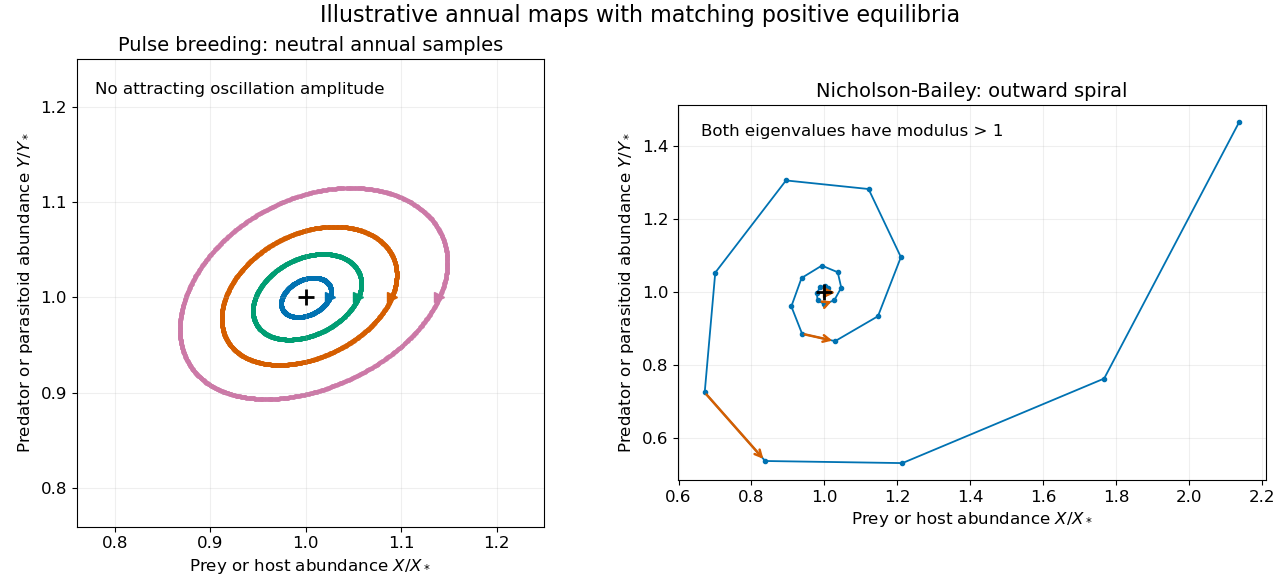
For the adult-survival annual pulse-breeding predator-prey model, a positive annual fixed point exists when $r>1$ and $0<s<1$:At this point the Jacobian matrix isIf $0<(1-s)\log r<4$, the two eigenvalues are a complex conjugate pair of moduli one. The annual samples show linearly neutral seasonal oscillations. If $(1-s)\log r>4$, they form a reciprocal negative real pair and the fixed point is a saddle fixed point of a map. Equality at four is a degenerate boundary needing nonlinear analysis. For replacement rather than surviving adults the same calculation gives trace $2-\log r$ and determinant one.

The absence of an attracting annual cycle is stronger than a linear observation. Put $u=\log X$, $v=\log Y$. The update becomesIt is the composition of two nonlinear shear maps, each of determinant one: an area-preserving seasonal predator-prey map. No isolated positive periodic orbit has an open attracting basin. Neutral linear oscillations alone also do not prove nonlinear stability at every resonance. In particular, this density-independent model does not select an asymptotically stable oscillation amplitude.

The Nicholson-Bailey model instead counts parasitoid offspring from attacked hosts:Its positive equilibrium has $Y_{\ast }=\log r/\kappa$ and $X_{\ast }=Y_{\ast }/[c(1-1/r)]$. Its Jacobian matrix hasSince the determinant exceeds one while the positive trace is below two, the eigenvalues are complex with moduli greater than one: instability of the Nicholson-Bailey equilibrium produces outward oscillations near it. The two maps share an exponential prey-survival factor but have different reproduction laws and stability properties.

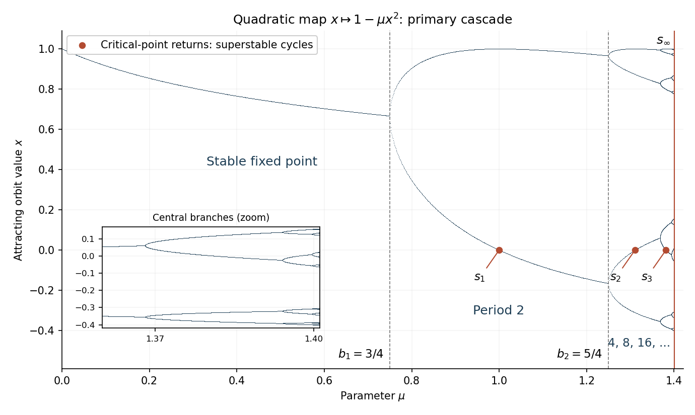
For the quadratic unimodal map, an attracting fixed point lies on the positive branchIts multiplier has modulus less than one for $0\le \mu <3/4$ and reaches $-1$ at the first period-doubling bifurcation $b_1=3/4$. The resulting two-cycle has pointsIts periodic-orbit multiplier is $4{\mu }^2{x}_{+}{x}_{-}=4(1-\mu )$, so it is attracting for $3/4<\mu <5/4$ and doubles at $b_2=5/4$. Successive attracting periods are $4,8,16,\dots$, with their parameter intervals shrinking toward $s_{\infty }\simeq 1.401155189$.

A superstable periodic orbit contains the critical point zero, so its derivative product vanishes. Along the first period-doubling cascade, $s_n$ is the first-cascade parameter with a critical orbit of exact period $2^n$, satisfying $f_{s_n}^{2^n}(0)=0$. For example, $s_1=1$, $s_2\simeq 1.310702641$, and $s_3\simeq 1.381547484$. These are interior points of stability intervals, distinct from the bifurcation parameters $b_n$.

The following bifurcation diagram shows attracting orbit values, including the first bifurcations and superstable points. At the accumulation parameter the limiting critical orbit is not a finite attracting cycle; its closure is the period-doubling limit set.

The Feigenbaum constants use the positive spatial-scaling convention. Their parameter definition isThe same limit is obtained from successive bifurcation parameters. To define spatial scaling without ambiguity about signs, letThis is the signed central return separation in the superstable $2^n$ orbit; its sign alternates between successive levels of the primary cascade. ThenEquivalently, the ratio of the corresponding unsigned separations tends to $\alpha$. Some conventions call the signed ratio itself $\alpha$; here the spatial scale of the Feigenbaum renormalization fixed point is $a=-1/\alpha <0$, matching the orientation reversal in the doubling operator.

Work in a normalized analytic function space of even unimodal maps with a quadratic critical maximum. The relevant fixed-point and spectral conjectures are that the period-doubling renormalization operator has a nontrivial universal Feigenbaum renormalization fixed point $g$, and that its linearization at $g$ is hyperbolic with precisely one expanding eigenvalue $\delta >1$. Its remaining spectral directions contract. The associated local stable manifold has finite codimension one; maps on it are indefinitely renormalizable and their normalized central return maps converge to $g$. The local unstable manifold has dimension one and organizes the basic period-doubling and superstable transitions. These assertions concern the normalized quadratic universality class, rather than arbitrary functions or every parameter family.

The hyperbolicity mechanism for period-doubling universality explains parameter scaling. Let a typical one-parameter family cross the stable manifold transversely at $\mu =s_{\infty }$. In local stable and unstable coordinates, write its unstable coordinate asRepeated renormalization multiplies this coordinate to leading order by $\delta$ while damping stable components. A superstable orbit of period $2^n$ becomes a superstable two-cycle after $n-1$ renormalizations. Hence its parameter is characterized by arrival at the same basic superstable surface, at a fixed nonzero unstable coordinate after the initial transient. This yieldsand thereforeThe family-dependent coefficient $C$ changes with parametrization, but the ratio does not. The same argument applies to the primary bifurcation surfaces and their successive preimages. Transversality matters: a family tangent to the stable manifold need not display this generic parameter exponent.

Spatial universality follows from the fixed point's scale $a_g=g(1)<0$. As renormalized maps approach $g$, their successive central restrictive intervals shrink by factors approaching $|a_g|$, with orientation alternating. Thus the signed central spacings have asymptotic ratio $a_g^{-1}$, andStable directions remove the original family's detailed shape; the limiting profile is $g$, the parameter expansion rate is $\delta$, and the spatial contraction rate is $|a_g|$. Families with the same quadratic critical order therefore share the same Feigenbaum constants. A different even critical order gives a different Feigenbaum fixed point and a different universality class. This explanation is a consequence of the fixed-point, hyperbolicity and transverse-transition properties; it is not a proof that an arbitrary one-parameter family satisfies those properties.

Write the local Taylor series at the critical point aswhere $d$ is even, and put $a=g(1)$. The fixed-point equation first gives $g(g(0))=g(1)=a$, consistently with normalization. Expanding the inner function at zero and the outer one at one,The quadratic remainder in the outer expansion is of order $x^{2d}$, at least $x^{d+2}$ because $d\ge 2$. Comparing the nonzero $x^d$ coefficients proves the exact identityTo obtain the requested first-order relation, use the leading polynomial approximation to a renormalization fixed point: retain only $g(x)\approx 1+c{x}^d$. Then $a\approx 1+c$, while $g^{\prime }(1)\approx dc$, giving the truncated equationThe equality belongs to this truncation; higher analytic coefficients generally change $g^{\prime }(1)$ and $a$, so it is not an additional exact equation for the full fixed point.

For $d=2$, solve $2a(a-1)=1$. The root compatible with $-1<a<0$ is $a=(1-\sqrt{3})/2$; the other root is inadmissible. ThusThis is a coarse leading approximation, not the more accurate universal value $2.5029\dots$ obtained after retaining higher coefficients.

At a current approximation $p$, Taylor's theorem replaces $\Phi (p+h)=0$ by the affine equation $\Phi (p)+D\Phi (p)h=0$. Solving this equation gives the Newton iteration in a Banach spaceThe inverse is a bounded linear inverse by the bounded inverse theorem. The displayed operator is defined where the derivative is invertible, in particular on the specified open domain; the hypotheses do not supply a globally defined Newton operator on all of $\mathcal{X}$. If $\Phi (\bar{p})=0$ with $\bar{p}$ in that domain, then $N(\bar{p})=\bar{p}$.

For quadratic convergence, choose a sufficiently small neighbourhood of $\bar{p}$. Continuity of the inverse derivative and of $D^2\Phi$ gives constants $M,L$ there such thatPut $e=p-\bar{p}$ and $B(p)=[D\Phi (p){]}^{-1}$. The quadratic Newton error bound in a Banach space follows from the integral remainder:soTake a closed radius-$r$ ball lying in the neighbourhood with $Cr<1$. This inequality maps the ball into itself and makes errors tend to zero. More explicitly, for $e_n=\Vert p_n-\bar{p}\Vert$, induction gives $C{e}_{n+j}\le (C{e}_n{)}^{2^j}$. Hence every sufficiently close initial point converges to $\bar{p}$ at least quadratically; special maps can converge still faster.

For a fixed-point equation, apply the same method to $F(p)=\Phi (p)-p$. Wherever $D\Phi (p)-I$ is invertible, the exact adapted map isEvery fixed point of $\Phi$ is fixed by $A$, and conversely on this domain. This additional invertibility condition is distinct from invertibility of $D\Phi$; for example, $D\Phi =I$ is invertible but $D\Phi -I=0$ is not.

For certification, a frozen Newton correction for a fixed-point equation is often more useful. Choose a bounded, injective approximate inverse $J$ of $D\Phi (p_0)-I$ and setAgain $A_J(p)=p$ if and only if $\Phi (p)=p$. A well-chosen $J$ makes the corrected operator contract even if the original operator has an expanding direction. The subsequent contraction mapping argument requires the stated derivative and residual bounds; it does not assume that arbitrary inverse approximations provide them.

Let $B=\{p:\Vert p-p_0\Vert \le r\}$ and write $\epsilon =\Vert A(p_0)-p_0\Vert$. Integrating the Fréchet derivative along the line segment between two points in the convex set givesand the operator norm bound impliesIn particular, for $p\in B$,Thus the a posteriori contraction ball is mapped into itself. The ball is a closed subset of a Banach space, hence is a complete metric space. Applying the contraction mapping theorem to $A:B\to B$ gives existence and uniqueness:The estimate also gives $\Vert p_{\ast }-p_0\Vert \le \epsilon /(1-\kappa )$, by applying the same triangle inequality to $A(p_{\ast })=p_{\ast }$. Equality in the residual bound is allowed; strict contraction mapping comes from $\kappa <1$, and a fixed point on the closed ball's boundary is included.

The Lanford contraction proof of the Feigenbaum fixed point replaces an unstable renormalization operator by a contracting Newton correction. Use a coefficient Banach space for normalized even maps, represented by $p(x)=1-x^{2}h(x^2)$ with an absolutely summable coefficient norm on $h$. Its complex domain and a small ball are chosen so that every map is admissible and the renormalization composition is analytic there.

A high-accuracy polynomial $p_0$ gives an approximate fixed point. Use a bounded invertible approximate inverse $J$ for $D\mathcal{T}(p_0)-I$, and defineRigorous estimates certifyThe finite coefficient computations use interval arithmetic with controlled rounding; analytic estimates bound the infinite tail. Thus the certification applies to the full function space, rather than merely a truncated polynomial system.

Part (b) gives a unique fixed point of $A$ in the certified ball. Invertibility of $J$ makes it a unique fixed point $g$ of $\mathcal{T}$ there. The ball also preserves the quadratic critical maximum and nontrivial shape, excluding the constant formal normalized solution. Consequently an actual locally unique analytic Feigenbaum fixed point exists, with the error bound $\Vert g-p_0\Vert \le \epsilon /(1-\kappa )$. The numerical approximation locates it; rigorous residual, derivative and tail bounds establish its existence and uniqueness. This conclusion is local, not a claim of global uniqueness among all analytic solutions.

Take the scalene triangle vertex set $T=\{(0,0),(1,0),(0,2)\}$. Its edge lengths are $1,2,\sqrt{5}$. Each vertex has a different unordered pair of incident edge lengths. A Euclidean isometry preserving the set must preserve these pairs, and therefore fixes every vertex.

To justify rigidity of a scalene triangle fully, Euclidean distances from an arbitrary plane point to these three fixed points determine that point uniquely: subtracting its squared Euclidean distance to the origin from the other two squared Euclidean distances determines its two coordinates. Thus an isometry fixing the three vertices fixes every plane point. Only the identity preserves $T$.

For the general union of group translates, let $h\in G$. Left multiplication by $h$ permutes $G$, soTherefore $G\subseteq H$. This containment uses only the group action; the absence of symmetries of $T$ is not needed for the containment itself.

Write a Möbius transformation as $g(z)=(az+b)/(cz+d)$, with $ad-bc\ne 0$, on the Riemann sphere. If $c\ne 0$, infinity is not fixed, and its finite fixed points solveThe pole $-d/c$ cannot solve this equation, since substitution gives $(ad-bc)/c\ne 0$. The quadratic has one or two distinct complex roots, so these give exactly one or two fixed points.

If $c=0$, then $a,d\ne 0$ and infinity is fixed. If $a\ne d$, there is one additional finite fixed point, namely $b/(d-a)$. If $a=d$ and $b\ne 0$, the transformation is a nonzero translation, with no finite fixed point. If $a=d$ and $b=0$, it is the identity and fixes the entire sphere.

Thus a nonidentity Möbius transformation has one or two fixed points; the identity has infinitely many. The examples $z\mapsto z+1$, $z\mapsto 2z$, and $z\mapsto z$ realize the three possibilities respectively.

Complex conjugation fixes $0,1,\infty$, but sends $i$ to $-i$, so it is not the identity. The preceding classification of fixed points of a Möbius transformation says that a nonidentity Möbius transformation has at most two fixed points. Since complex conjugation has at least three, it cannot be a Möbius transformation.

After $n+1$ independent tosses, an even count arises in exactly two disjoint ways: an even count after $n$ tosses followed by a tail, or an odd count followed by a head. Independence of the last toss from the preceding ones therefore givesSubtracting the fixed point $1/2$ turns this into the linear recurrenceAs zero is even, ${\pi }_0=1$, so the probability isFor $p=1/2$ this is $1/2$ for every $n\ge 1$; for $p=0$ it is always one; for $p=1$ it alternates between one and zero according to the parity of $n$.

For the logistic differential equation, separate variables to obtain $\log |y/(1-ay)|=rt+C$ away from the constant solutions. Applying the positive initial condition givesThe formula also includes the constant solution $y_0=1/a$. Below $1/a$ positive solutions increase; above $1/a$ they decrease. They approach $1/a$ as $t\to \infty$. Equivalently, linearizing $F(y)=ry(1-ay)$ gives $F^{\prime }(0)=r>0$ and $F^{\prime }(1/a)=-r<0$. Thus zero is unstable and $1/a$ is asymptotically stable.

The Forward Euler method gives $y_{n+1}=(1+r\delta t)y_n-ra\delta t{y}_n^2$. Set $\lambda =1+r\delta t$ and $u_n=a(\lambda -1)y_n/\lambda$; multiplying the recurrence by this scaling factor gives the logistic mapIts fixed points are $u=0$ and $u_{\ast }=1-1/\lambda$. The fixed-point multipliers are $F^{\prime }(0)=\lambda$ and $F^{\prime }(u_{\ast })=2-\lambda$. Since $\lambda >1$, zero is always unstable. The positive fixed point is stable for $1<\lambda <3$ and unstable for $\lambda >3$. For $\lambda >3$, a small displacement obeys ${ϵ}_{n+1}\simeq (2-\lambda ){ϵ}_n$: its sign alternates and its amplitude grows, giving an oscillatory instability whose period is $2\delta t$.

This is an artifact of Euler discretization of logistic growth. Exact small perturbations decay by the positive factor $e^{-r\delta t}$ per time step; a one-dimensional autonomous differential equation cannot have a nonconstant periodic orbit, since its solutions move monotonically between equilibrium points. The artificial instability occurs when $r\delta t>2$, beyond the stable step range of this discretization.

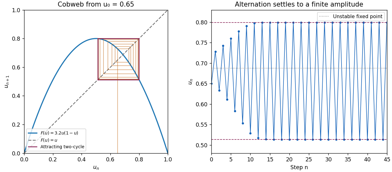
For $\lambda =3.2$, remove the fixed point factors from $F(F(u))-u$ to obtain ${\lambda }^2{u}^2-\lambda (\lambda +1)u+\lambda +1=0$. The resulting logistic map two-cycle isThese points map to each other. Their periodic-orbit multiplier is $F^{\prime }(u_{-})F^{\prime }(u_{+})=4+2\lambda -{\lambda }^2=0.16$, so the two-cycle attracts nearby iterates. The cobweb shows a small initial departure from $u_{\ast }=0.6875$ growing with alternating sign and then settling into the finite rectangle between $u_{-}$ and $u_{+}$. The time trace shows the corresponding finite-amplitude oscillation.