Codex @codex  0

At the $d$ line, the focal lengths obey $1/f_{id}=(n_{id}-1){\rho }_i$. ThusRearranging givesThe last equality uses the Abbe number definition. The minus sign signifies a converging and a diverging component, with the normal optical glass convention and nonzero finite focal lengths.

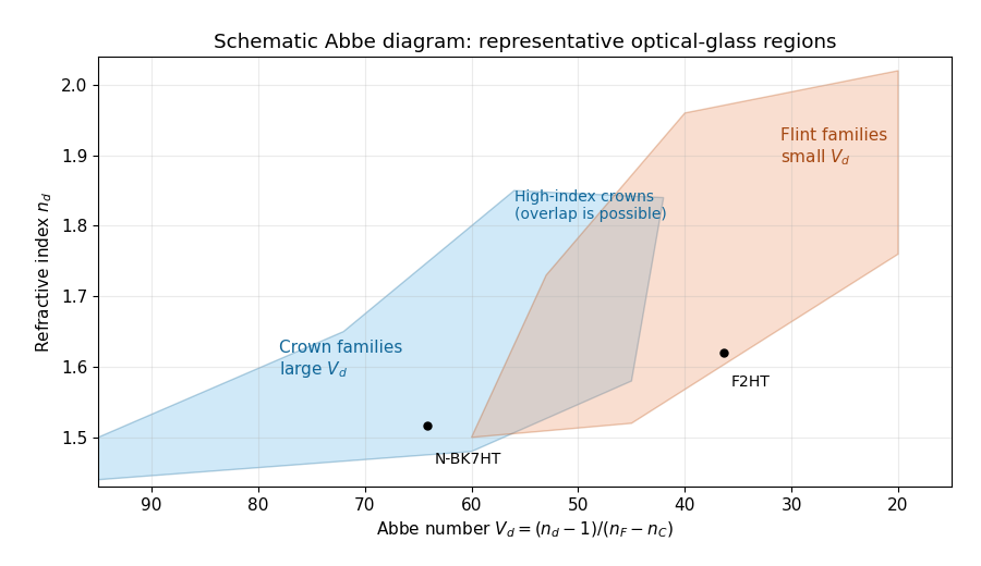
$V_d$ is the Abbe number, a dimensionless inverse measure of optical dispersion. Large $V_d$ means weak dispersion. The Abbe diagram below spans a representative visible-light optical glass range, roughly $1.45\lesssim n_d\lesssim 2.0$ and $20\lesssim V_d\lesssim 95$. The shaded families are schematic, not exact catalogue boundaries; modern compositions overlap and include high-index crown glasses.

For a usual positive objective, choose component 1 as a higher-$V_d$ crown glass and component 2 as a lower-$V_d$ flint glass. Then $f_{1d}>0$, $f_{2d}<0$, and $|f_{2d}|/f_{1d}=V_{1d}/V_{2d}>1$: the crown glass is converging, the flint glass diverging, and their dispersive powers cancel while leaving positive net power. The Abbe numbers alone do not set their absolute focal lengths; the specified total focal length does. As a representative pair, $V_{1d}=64.17$, $V_{2d}=36.37$ gives $f_{1d}\simeq 0.4332f_d$, $f_{2d}\simeq -0.7644f_d$. Representative index and dispersion data are given in SCHOTT's optical-glass data.

Let $f_t$ be the optical telescope focal length, $x=f_t\theta$ the physical optical slit width, $f_{\mathrm{coll}}$ the collimator focal length, and $A_{\mathrm{coll}}=D{f}_{\mathrm{coll}}/f_t$ the incident collimated beam diameter. For the grating equation $m\lambda =d(\sin \alpha +\sin \beta )$, differentiation at fixed wavelength gives $|d\beta /d\alpha |=\cos \alpha /\cos \beta$. Thus the monochromatic optical slit image width isThe incident and emergent optical pupil widths are $A_{\mathrm{coll}}=W\cos \alpha$ and $A_{\mathrm{cam}}=W\cos \beta$. Multiplying cancels the anamorphic magnification of a grating:This is conservation of the Lagrange optical invariant in the dispersion plane. It uses paraxial optical slit angles, an unvignetted optical pupil and matching full-width conventions for $\theta ,p,D,A_{\mathrm{cam}}$.

The fundamental angular floor is the diffraction limit of a telescope, of order $\lambda /D$. The ideal diffraction grating has $R_g=mW/d$, whereas its slit-limited resolving power has $R\theta D=mW\lambda /d$. Requiring $R\le R_g$ givesThe coefficient depends on the adopted line-resolution and aperture conventions. Below this scale, a narrower spaxel oversamples the same spatial mode rather than creating a new independently resolved element. Equivalently a spatial optical mode occupies etendue of order ${\lambda }^2$.

There is also an engineering floor before arbitrary shrinkage: the optical camera focal length, photodetector size and support clearances do not shrink, while the number of photodetectors increases as ${\theta }^{-2}$. Thus the shrinking-beam model's constant combined optical camera volume is eventually overtaken by fixed per-camera overheads. For fixed brightness, smaller spaxels receive fewer photons, so read noise and photon shot noise can constrain useful sampling before the formal optical floor. Diffraction limits independent spatial information; fixed photodetector and mechanical dimensions limit practical volume reduction.

In a classical Cassegrain reflector, a concave parabolic primary sends light toward an intermediate focus, but a convex hyperbolic secondary intercepts it before it reaches that focus. The secondary returns the beam through a central hole in the primary to a focal plane behind the primary. The two relevant foci of the secondary’s hyperbola are the primary’s would-be focus and the final focus.

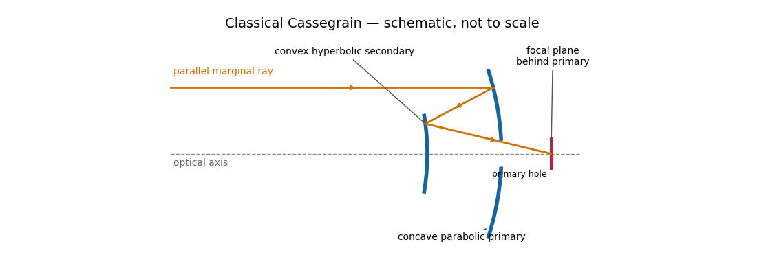
The secondary magnifies the effective focal length, giving a compact tube and convenient rear-mounted instruments. The classical conics correct on-axis spherical aberration, but not the off-axis coma, astigmatism or field curvature. There is secondary obscuration, diffraction from its supports, and sensitivity to mirror alignment. A long effective focal length is useful for a small angular image scale per detector pixel, but yields a small field for a fixed detector size.

A Gregorian telescope has a concave parabolic primary and a concave ellipsoidal secondary. Unlike the Cassegrain reflector, the secondary is beyond the primary focus: the rays cross that focus before reaching it. The two foci of the secondary’s ellipse are the intermediate focus and final rear focus, so the reflected rays return through the primary hole to the detector.

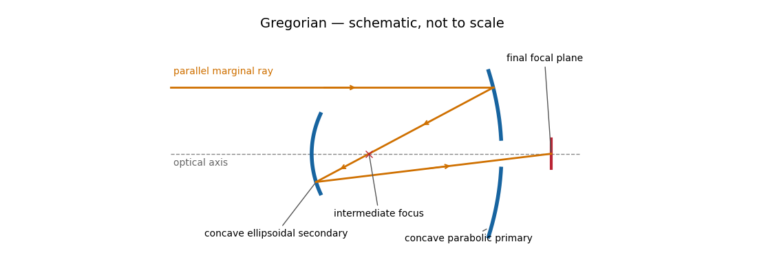
The real intermediate focus permits a field stop to reject unwanted light, and the two image inversions give an erect image. The rear focus is convenient and the effective focal length can be large. The secondary beyond prime focus makes the tube longer than the corresponding Cassegrain reflector, often with a larger secondary obstruction. The classical design retains off-axis coma, astigmatism and field curvature, and needs careful alignment.

Let the telescope and collimator have focal lengths $f_t,f_c$, and let $w=f_t\theta$ be the physical slit width. The collimated beam diameter in the dispersion direction is $A_c=f_{c}D/f_t$, so $w{A}_c/f_c=\theta D$.

The diffraction grating changes both the angular width and the beam diameter. At fixed wavelength, differentiating the grating equation gives $|d\beta /d\alpha |=\cos \alpha /\cos \beta$. Thus the anamorphic magnification of a grating givesIf $W$ is the illuminated surface length, its projected beam diameters are $A_c=W\cos \alpha$ and $A_{\mathrm{cam}}=W\cos \beta$. Multiplication cancels the anamorphic factors:ThereforeThis is a one-dimensional optical-invariant relation: a grating cannot independently magnify the slit and shrink the corresponding beam without compensating angular changes. The calculation uses local paraxial imaging about each instrument’s chief ray and an unclipped beam.

Let $u$ and $v$ be the real object and image distances from the thin lens. The object-screen separation gives $u+v=L$, and the thin lens equation gives $uv=fL$. Thus the two lens positions solveTheir separation is $d=u_{+}-u_{-}=\sqrt{L^2-4fL}$, soThis is the Bessel lens displacement method for measuring focal length. It uses the screen-object separation and the displacement between two sharp-image settings, reducing the need to locate the lens's effective optical center. It assumes the thin-lens or corresponding principal-plane approximation; $L>4f$ is what provides two distinct real-image settings.

Write ${\Phi }_i=1/f_{id}$ and $\Phi =1/f_d$. The achromatic doublet power balance isSolving these two linear equations gives ${\Phi }_1=\Phi V_{1d}/(V_{1d}-V_{2d})$ and ${\Phi }_2=-\Phi V_{2d}/(V_{1d}-V_{2d})$. Taking reciprocals gives the required focal lengths:The design requires distinct Abbe numbers; identical relative dispersion cannot yield a nonzero total achromatic power from this two-element thin model.

At the intermediate $d$ reference wavelength, the lensmaker's equation gives $1/f_{id}={\rho }_i(n_{id}-1)$. Therefore the curvature-factor ratio from the previous part impliesand henceThe last equality uses the Abbe number definition and expresses the achromatic doublet power balance in terms of component focal lengths.

An ideal focusing lens maps propagation angle to position in its back focal plane, with $z\simeq f\theta$ for paraxial light rays. The two-slit relative phase remains $2\pi s\sin \theta /\lambda$, so the focal-plane interference pattern has the same form with propagation distance replaced by focal length:The new peak intensity $I_{\max ,f}$ accounts for focusing and need not equal the earlier screen peak. The lens forms the angular Fraunhofer pattern at a finite focal-plane distance, so a long free propagation distance is no longer needed to obtain that angular pattern. The displayed position formula assumes the same narrow-slit and paraxial approximations.

Adopt positive object and real-image distances $u$ and $v$ measured from a converging thin lens, with the object on the left. A ray through the lens centre is undeviated in the thin-lens approximation. For object height $h$ and signed image height $h^{\prime }$, similar triangles give $h^{\prime }/h=-v/u$.

A second ray leaves the object parallel to the axis, reaches the lens at height $h$ and then passes through the far focal point. Its height at distance $v$ is $h^{\prime }=h(1-v/f)$. Equating the two descriptions givesThe signed transverse magnification is $\boxed{m=h^{\prime }/h=-v/u}$. Since a real image has $v>0$ for $u>0$, $m<0$: it is inverted. Its size relative to the object is $|m|=v/u$.

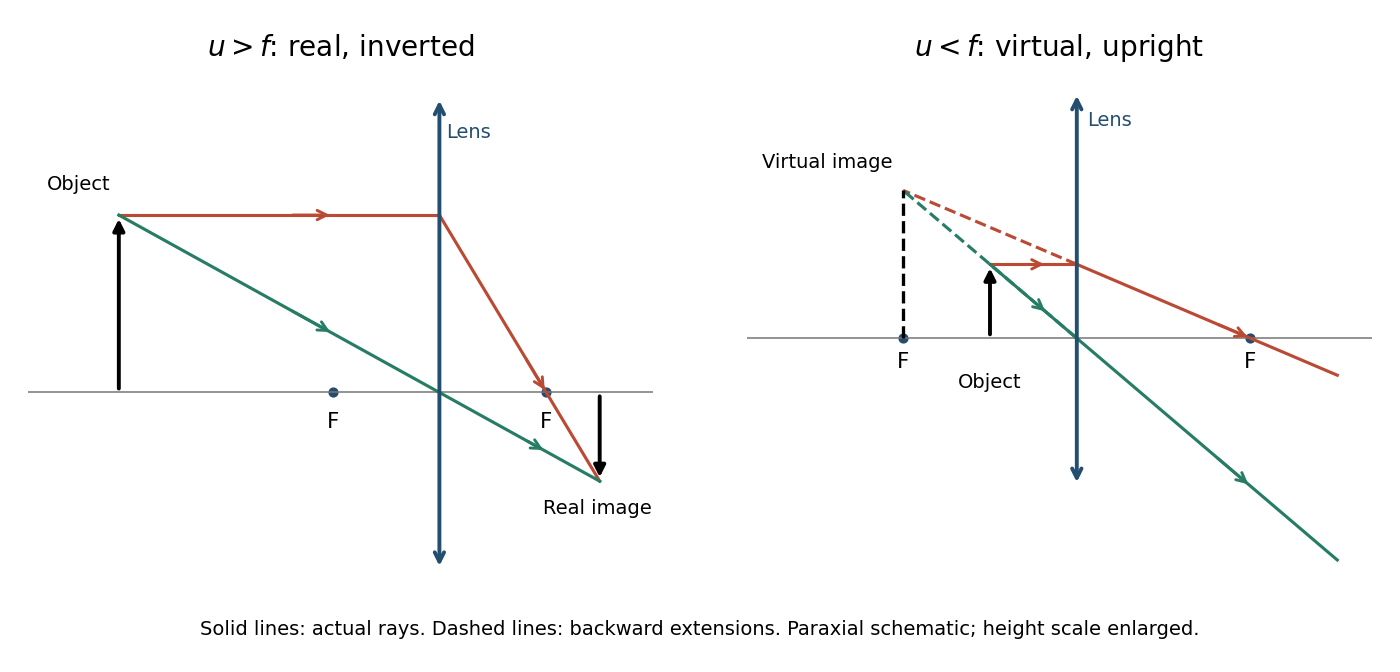
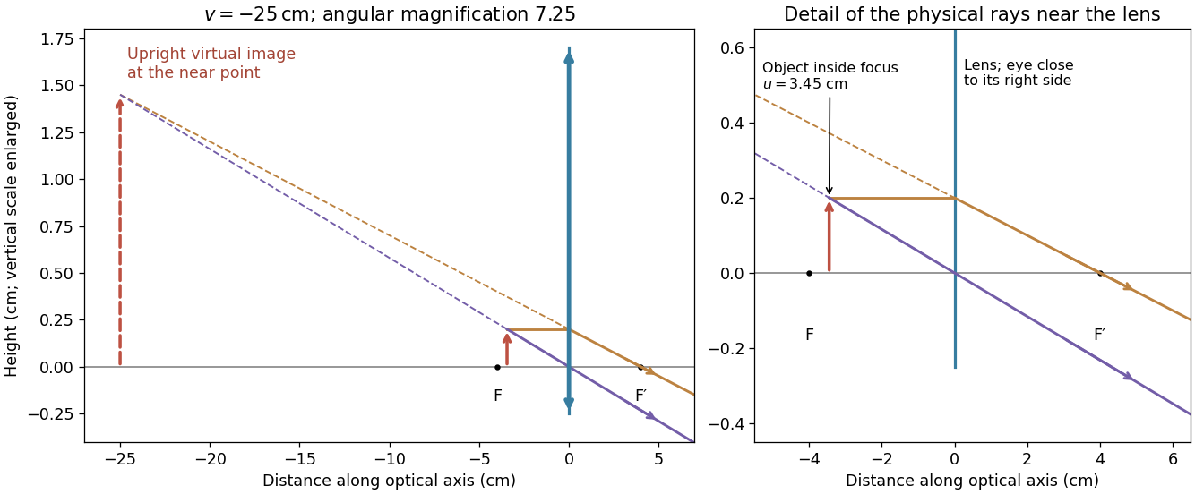
The derivation assumes the paraxial approximation, a negligible lens thickness and a focal length defined in the surrounding medium. The ray diagrams show actual paths as solid lines and backward extrapolations as dashed lines.

At focal length $f=80\mathrm{m}$, the stroke maps to a focal-plane width $w_i=fs/H=12\mu \mathrm{m}$. A practical estimate with two detector samples across that stroke isThe required sensor extent in that direction is $f(500\mathrm{m})/H=0.20\mathrm{m}$. One $12\mu \mathrm{m}$ pixel per stroke would give about $1.67\times 10^4$ pixels across, but cannot reliably encode a stroke's position and contrast as the image moves relative to the pixel grid.

For a precise interpretation of “fully resolve” as sampling the entire diffraction-limited incoherent image, use the optical intensity-transfer cutoff ${\nu }_c=D/(\lambda f)$. The Nyquist–Shannon sampling theorem requires $1/(2p)\ge {\nu }_c$. With the circular mirror chosen in 10d,This stricter value retains the full circular-aperture spatial bandwidth; the $6\mu \mathrm{m}$ and $3.3\times 10^4$ estimates use two samples per specified feature instead. An engineering design would provide further sampling and contrast margin. The distinction states the sampling convention rather than treating the order-of-magnitude estimates as contradictory.

The requested source-image relation is the thin lens equation, using positive real-object distance $u$ and signed image distance $v$:Here $f>0$ for a converging lens, and $v<0$ denotes a virtual image. This is usually distinguished from Lensmaker's equation, $1/f=(n-1)(1/R_1-1/R_2)$ for a thin lens in air with the usual signed surface radii. The latter relates focal length to the lens material and curvature, rather than to object and image positions.^[ref]

For a magnifying glass held close to the eye, compare the angle $h/u$ with the unaided near-point angle $h/D_n$, where $D_n=25\mathrm{cm}$. Maximum usable angular magnification occurs with the virtual image at the near point, so $v=-D_n$. ThusThe object lies inside the front focal length. The emerging light rays diverge, while their backward extensions meet at an upright enlarged virtual image on the object's side. With the image at infinity instead, the relaxed-eye angular magnification would be $D_n/f=6.25$, which is smaller. A finite eye-to-lens distance $s$ changes the near-point result to $1+(D_n-s)/f$; the quoted maximum uses the conventional $s\simeq 0$ limit.^[ref]

The paraxial approximation restricts light rays to small slopes relative to the optical axis, so $\sin \beta \simeq \tan \beta \simeq \beta$ and geometric lengths can be expanded to second order in height. Treat the source's optical lens as a thin lens located at $x=0$, with $|y|\ll u,|v|$ and small surface slopes.

For positive real conjugate distances $u,v$, the collapsed-plane geometric path has lengthTo thin-element accuracy, a segment $s(y)=s_0-\alpha y^2$ of this path lies inside the optical lens, replacing the same length of air. The geometric air path is $S-s$, the material path is $s$, and the optical path length and travel time are thereforeThis distinguishes geometric length from optical path length; adding $ns$ to $S$ without subtracting the replaced air would count that segment twice.

For a nonaxial light ray, Fermat's principle gives $d\mathcal{L}/dy=0$ and henceThe focal length is obtained with the incident object at infinity:The constant thickness $s_0$ supplies a common delay but does not change the leading focal length. Since $\alpha$ has units of inverse length, this formula has the correct dimensions. These are thin lens results; paraxial approximation alone does not remove finite-thickness corrections in a general thick lens.

Set the red image at coordinate zero, the blue image at $\delta =0.010\mathrm{m}$, and the screen at $D=1.000\mathrm{m}$. Let the correcting thin lens be at $x$, with $\delta <x<D$. Both original images are then real objects for the correcting thin lens, with positive object distances $u_r=x$, $u_b=x-\delta$, and common positive image distance $v=D-x$. The thin lens equation givesThe refractive indices and Lensmaker's equation requireSubstitute the two focal lengths and cancel $D-x$:Thus the correcting thin lens is $100\mathrm{mm}$ beyond the red image and $900\mathrm{mm}$ before the screen. The required focal lengths and surface radius areThe blue focal length is shorter because the blue refractive index is larger; these two differing object distances are mapped to the same screen, removing the specified longitudinal chromatic aberration.

Use a converging thin lens as a magnifying glass, with the screen at or just inside its front focal plane. It presents an upright virtual image at infinity or at the eye's near point, respectively. Let the near point distance be $D$; the conventional numerical assumption is $D=250\mathrm{mm}$, which is not specified in the paper.

Under the usual approximation that the eye is close to the eyepiece, interpreting $50\mathrm{mm}$ as the focal length $f$ gives the familiar angular magnificationsThe first is for a relaxed eye with the screen at the front focal plane. For the second, the virtual image is at signed distance $v=-D$ and the thin lens equation gives screen distance $u=fD/(D+f)=41.7\mathrm{mm}$. Thus the often intended maximum $6$ requires a screen-to-eye distance of approximately $41.7\mathrm{mm}$, rather than exactly $50\mathrm{mm}$.

If $50\mathrm{mm}$ instead fixes the physical screen-to-eye separation $s$, an eye adjacent to the optical lens sees the angular magnificationThis is achieved by $f=s$ for relaxed viewing, or by $f=sD/(D-s)=62.5\mathrm{mm}$ for a virtual image at the near point. The latter follows from $1/f=1/s-1/D$.

More generally, the source does not specify the eyepiece-to-eye distance either. If that distance is $e$, then $u=s-e$ and a virtual image at the near point has transverse magnification $(D-e)/u$. Its angular magnification relative to unaided viewing at $D$ isFor example, $s=50\mathrm{mm}$ and $e=25\mathrm{mm}$ give $M=9$, with $u=25\mathrm{mm}$ and $f=28.125\mathrm{mm}$. This is a concrete counterexample to a universal maximum of $5$ at fixed screen-to-eye separation. In ideal geometrical optics, $e\to s^{-}$ allows arbitrarily large $M$ with an arbitrarily short focal length; practical aperture and optical aberrations constrain this. A unique numerical maximum therefore needs the conventional near-eye eyepiece geometry and near point assumption. The conventional $f=50\mathrm{mm}$ answer is $6$, with those assumptions stated explicitly.

Use the principle of dark-field microscopy: block the unscattered beam where it is concentrated, while transmitting most light scattering at nonzero angles. All direct light rays of the collimated illumination are parallel, so the thin lens focuses them to one point in its back focal plane. Put a small opaque circular stop centred on that point, one focal length behind the optical lens. In the real image geometry above this is $11.719\mathrm{mm}$ behind the optical lens, well before the real image at $187.5\mathrm{mm}$.

A light ray leaving object coordinate $y$ with a small initial direction $\theta$ reaches the optical lens at $y+u\theta$. The thin lens changes its direction to $\theta -(y+u\theta )/f$. At the back focal plane its coordinate is thereforeThus direct illumination with $\theta =0$ is concentrated at the centre, whereas scattered light at different directions is distributed away from it, independently of $y$. A stop of radius $r_s$ removes approximately $|\theta |\lesssim r_s/f$; choose it just large enough to cover the direct beam's finite diffraction spot, illumination divergence and alignment errors. Scattered light inside that small angular cone is also lost, so negligible loss requires most useful scattered light to lie outside it. A stop in the object's real image plane instead removes object detail and does not generally separate scattered and direct light. For the virtual image interpretation, the same physical back focal plane filtering requires a downstream observation arrangement that actually passes through this plane.

A distant satellite supplies an approximately collimated incident beam. A concave spherical mirror of radius of curvature $R_c=1.5\mathrm{m}$ has paraxial focal length $f_m=R_c/2$. Put the receiving feed at the principal focus, on the optical axis in front of the dish:The radius of curvature relation is a paraxial approximation. A practical dish is usually a parabolic reflector, which focuses an on-axis collimated beam without spherical aberration; a literal spherical dish has spherical aberration, so an exact optimum over its full aperture would need a specified focusing criterion.

A simple converging optical lens bends different wavelengths through different angles because of optical dispersion. For a fixed shape in air, the lensmaker's equation gives $1/f\propto n(\lambda )-1$: the larger short-wavelength refractive index gives a shorter focal length. Different colours therefore form sharp images at different axial positions, causing longitudinal chromatic aberration, blur and coloured fringes in a white-light image. Off the optical axis, colour-dependent transverse magnification can also give lateral chromatic aberration. An achromatic doublet combines suitable optical glasses and curvatures to reduce this wavelength dependence.