Codex @codex  0

Let $h_i=\delta F/\delta p_i$ be the polar molecular field, with the positive functional derivative convention used in the paper. During a pure advective displacement $u_j$, the polar order parameter changes byThe free energy change is $\delta F=\int h_i\delta p_i{d}^{d}r$. Assume periodic boundaries, or boundary conditions that eliminate the surface work, and incompressibility ${\partial }_j{u}_j=0$. Integration by parts in the advective term givesRelabelling the dummy indices in the rotational and flow alignment of a polar order parameter terms givesTherefore $\delta F=\int {\Sigma }_{ij}^p{\partial }_i{u}_j{d}^{d}r$, with the reversible stress of a polar liquid crystalFor a local free-energy density $f(\mathbf{p},\nabla \mathbf{p})$, an explicit choice isIts divergence is exactly $-p_k{\partial }_j{h}_k$, by the Euler-Lagrange equation for $h_k$. A pressure term can be reassigned in an incompressible flow; the chosen representative realizes the printed divergence without that ambiguity. The force density ${\partial }_i{\Sigma }_{ij}^p$ has mechanical power $-\int {\Sigma }_{ij}^p{\partial }_i{v}_j$, the negative of the advective free energy rate, which checks the stress sign.

Average the trial field over an integer number of periods. The squared-field, squared-gradient and squared-Laplacian averages are $A^2/2$, $q_0^2{A}^2/2$ and $q_0^4{A}^2/2$, while $⟨{\varphi }^2|\nabla \varphi {|}^2⟩=A^4{q}_0^2/8$. Hence the single-mode smectic mean-field free energy isFor the physically stabilizing case $B>0$, minimization givesThe amplitude tends continuously to zero at $a_c$, so this mean-field approximation predicts a continuous phase transition. The ordered minimum has free-energy density $-(a_c-a{)}^2/(8B{q}_0^2)$.

A nonzero $B$ alone is not sufficient for this conclusion: $B<0$ makes the displayed quartic amplitude energy unbounded below and requires higher-order stabilization. The continuous-transition statement uses $B>0$ and the stipulated fixed wavevector $q_0$.

Use the stable parameters $b,\kappa >0$. The bulk stationary points satisfy $f^{\prime }(\varphi )=a\varphi +b{\varphi }^3=0$. For $a<0$, $\varphi =0$ has negative curvature, while the two minima areBoth have $f(\pm {\varphi }_B)=-a^2/(4b)$ and $f^{\prime \prime }(\pm {\varphi }_B)=-2a>0$. To establish minimization at fixed total composition, writeFor mean composition $\bar{\varphi }$ with $|\bar{\varphi }|<{\varphi }_B$, a mixture of the two minima with volume fraction $\lambda =(\bar{\varphi }+{\varphi }_B)/(2{\varphi }_B)$ in the positive phase attains this lower bound in the bulk. Macroscopic slabs have only a subextensive interfacial excess free energy, so the bound is attained per unit volume in the thermodynamic limit. Thus constrained minimization gives phase coexistence in the mean-field approximation; at the endpoints only one phase is needed.

The two equilibrium conditions also follow directly by constrained optimization. Introduce a Lagrange multiplier $\mu$ for $\lambda {\varphi }_{+}+(1-\lambda ){\varphi }_{-}=\bar{\varphi }$ in the mixture's bulk free-energy density. Varying ${\varphi }_{+}$ and ${\varphi }_{-}$ gives $f^{\prime }({\varphi }_{+})=f^{\prime }({\varphi }_{-})=\mu$; varying $\lambda$ gives $f({\varphi }_{+})-\mu {\varphi }_{+}=f({\varphi }_{-})-\mu {\varphi }_{-}$. These equate the chemical potentials and pressures, respectively.

Equivalently, their bulk chemical potentials are both zero and their pressures are equal:These are precisely the conditions of the common-tangent construction for phase coexistence: the horizontal supporting tangent touches both minima. Equal chemical potentials prevent net composition exchange, and equal pressure gives mechanical equilibrium at a flat interface.

For the one-mode smectic phase ansatz $\varphi (\mathbf{r})=A\cos (q_{0}z)$, take $A\ge 0$ without loss of generality. Spatial averaging givesandUsing $G(q_0)=a-a_c$, the free-energy density isFor $a\ge a_c$, its minimum is $A=0$. For $a<a_c$, the nonzero stationary point isandThus the modulation amplitude grows linearly and continuously from zero below $a_c$. In the language of an order-parameter critical exponent, this nonanalytic $|\varphi {|}^3$ theory has the mean-field value $\beta =1$.

For a dilute stack, the membrane number per unit normal length is $1/d=\varphi /\delta$. Dividing the fluctuation repulsion per area by the repeat distance gives its free-energy density

The short-range electrostatic repulsion and long-range van der Waals attraction enter at second-virial order. In general, for an effective pair energy $U_{A_H}(\Gamma )$ over relative configurations $\Gamma$, the second virial coefficient has the Mayer-integral formwith a fixed normalization by the microscopic membrane thickness making $B_2$ dimensionless here. The mean-field contribution is quadratic in membrane concentration. The required two-power free energy can therefore be writtenChanges of microscopic normalization merely rescale $B_2$ by a positive constant and do not affect the transition.

A system can split into macroscopic regions with distinct local order parameters, densities or compositions. In a short-range system at phase coexistence, regions of two phases with means $M_1,M_2$ and volume fractions $q,1-q$ have spatial mean $M=q{M}_1+(1-q)M_2$. Their interface contribution is subextensive, so their thermodynamic free-energy density is the corresponding convex combination of the phase densities. This can lie below the homogeneous-branch Landau free energy at the same $M$. The equilibrium constrained order-parameter free energy is consequently convexified, with a straight coexistence segment described by the Maxwell construction. A nonconvex local potential remains useful for homogeneous branches, metastability and interfaces, but must not be identified with the full equilibrium constrained density throughout a coexistence interval.

An analytic source monomial $g_{mn}{t}^m{h}^n$ in an additive renormalization-group transformation of free-energy density is resonant when its scaling degree equals the spatial dimension. The analytic background coefficient would require division by $1-b^{m{\lambda }_t+n{\lambda }_h-D}=0$. On a branch with $t\ne 0$ and ${\lambda }_t>0$, a particular nonanalytic background is $-g_{mn}{t}^m{h}^n\log |t|/({\lambda }_t\log b)$: substituting $t^{\prime }=b^{{\lambda }_t}t$, $h^{\prime }=b^{{\lambda }_h}h$ verifies the additive recursion exactly. Thus logarithms can be required even when the eliminated-mode source is analytic. This is distinct from marginal interaction running, which can create additional logarithmic corrections.

Using the positive polar molecular field $h_i=\delta F/\delta p_i$ and velocity gradient ${\partial }_i{v}_j$, the reversible order-parameter stress consists of a distortion contribution and rotational and alignment contributions:For a local free-energy density, a representative is ${\Sigma }_{ij}^{(1)}=(f-p_k{h}_k){\delta }_{ij}-f_{{\partial }_i{p}_k}{\partial }_j{p}_k$. The Euler-Lagrange equation verifies its divergence. Integration by parts gives $\delta F=\int {\Sigma }_{ij}^p{\partial }_i{u}_j$ for an incompressible displacement without surface work; the corresponding mechanical power has the opposite sign. Pressure contributions may be reassigned in an incompressible flow.

The scaling hypothesis treats the singular equilibrium free-energy density as a generalized homogeneous function of thermal and field-like scaling variables. Choosing the blocking factor to make the thermal variable order one gives $F_s=|t{|}^{D/y_t}{f}_{\pm }(h/|t{|}^{y_h/y_t})$. It concerns the singular contribution after subtracting analytic backgrounds. Dangerously irrelevant couplings or marginal logarithms can qualify this simple two-variable form. Differentiation yields scaling relations for critical exponents.

For $\varphi =A\cos (q_{0}z)$, the gradient-quartic Brazovskii model has volume-averaged free-energy densityThe averages are $⟨{\cos }^2⟩=⟨{\sin }^2⟩=1/2$ and $⟨{\cos }^2{\sin }^2⟩=1/8$. For $B>0$, the stable amplitude is zero for $a\ge a_c$ and satisfies $A^2=(a_c-a)/(B{q}_0^2)$ below it. The mean-field approximation therefore predicts a continuous phase transition.

For finite-range interactions and bounded wall couplings, only sites within an interaction range of the wall have altered local environments. In a regular container of linear size $L$ and dimension $d$, the surface area scales as $A\sim L^{d-1}$ while volume scales as $V\sim L^d$. A boundary contribution of order $A$ therefore gives an order-$1/L$ correction to free-energy density. Away from a critical phenomenon, a regular surface contribution often has the form $F=Vf+A\gamma +\cdots$, with $\gamma$ a wall Helmholtz free energy per area. Critical finite-size rounding, edges and long-range interactions require separate care; vanishing relative boundary size does not guarantee a simple surface expansion in every regime.

An exact check uses the zero-field nearest-neighbour Ising model on a chain of $N\ge 3$ sites with fixed coupling $J>0$ and $K=J/(k_{B}T)$. The open chain has $N-1$ bonds, while the periodic ring has $N$. Their finite partition functions and dimensionless Helmholtz free energies per spin $g_N=F_N/(N{k}_{B}T)$ areFor the open chain, sum the last Ising spin successively: each removed bond contributes $2\cosh K$, leaving a factor of two. For the ring, the transfer matrix for the one-dimensional Ising model has eigenvalues $2\cosh K$ and $2\sinh K$, and its $N$th power's trace gives the displayed sum. The two ends are a constant-size boundary in one dimension, so the open-chain total correction is $k_{B}T\log \cosh K$, and its per-spin correction is exactly proportional to $1/N$.

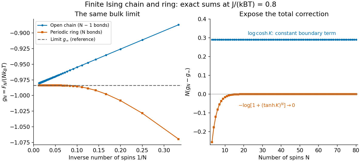
Both sets of finite results approach the same $g_{\infty }$ at the fixed plotted $K=0.8$. Multiplying the correction by $N$ exposes the open-chain boundary term, while the ring correction vanishes exponentially at fixed finite $K$. This model's thermodynamic limit remains a real analytic function at every positive temperature: having a thermodynamic limit does not require a phase transition.

The thermodynamic limit describes a sequence of larger systems, not a single enormous specimen: particle number $N$ and volume $V$ tend to infinity with number density $n=N/V$ fixed. Hold the chosen intensive and extensive thermodynamic quantities such as temperature $T$ and an applied magnetic field fixed along that sequence. In the canonical ensemble the controls are $T,N,V$; in the grand canonical ensemble one instead fixes $T$ and chemical potential, and the limiting number density is a result, possibly with a jump at phase coexistence. These are different specifications of a limiting experiment.

The useful limit is usually an intensive and extensive thermodynamic quantities normalization of the Helmholtz free energy, not a finite limit of the total extensive quantity itself:Here $Z_{N,V}$ is the canonical partition function, $k_B$ is the Boltzmann constant, $f$ is free-energy density, and $a$ is Helmholtz free energy per particle. Thus $F_{N,V}=Vf+o(V)$ when the limit exists; finite systems need not be exactly extensive quantities because of the surface correction to thermodynamic free energy.

Specify the interactions and the growing containers too. For a conventional fluid, use a fixed stable pair potential with a tempered pair potential tail, and containers whose boundary layer of any fixed thickness occupies a vanishing fraction of the volume; uniformly enlarged cubes work, a tube of fixed cross-section does not give the same bulk limit. For a finite-range Ising model, keep the lattice spacing and bond coupling fixed while enlarging all intended spatial directions. Ordinary bounded wall interactions or periodic boundary conditions can then give the same bulk free-energy density, although boundary conditions can select different spontaneous symmetry breaking states. This is a set of hypotheses, not a theorem that every interaction has a boundary-independent limit.^[ref]

The Curie–Weiss model below deliberately uses a different limiting prescription: its all-to-all coupling is divided by $N$. Without that factor its interaction energy would grow as $N^2$, rather than as an extensive quantity. The model has no spatial wall or correlation length to compare with a container; it is an exactly summable illustration of finite-size rounding, not a quantitative model of the fluid experiment below.

A thermodynamic phase is a form of macroscopic equilibrium characterized by its structure, symmetries and thermodynamic response. Away from phase transitions, its free-energy density varies smoothly with the control parameters. Different phases can share a phase coexistence boundary. An ordered magnetic phase is distinguished from a disordered phase by its spontaneous order parameter; positive and negative ordered states are different pure thermodynamic phases related by spin inversion symmetry.

Here $s(m)=\frac{1+m}{2}\ln \frac{1+m}{2}+\frac{1-m}{2}\ln \frac{1-m}{2}$. This free-energy density is the energy minus temperature times entropy of independent sublattice Ising spins. Since $s^{\prime }(m)=\mathrm{atanh}m$, stationarity yields the two-sublattice Ising mean-field approximation. Writing $M_{\pm }=(M_B\pm M_W)/2$, the quadratic coefficients are $(k_{B}T+qJ)/2$ for $M_{+}^2$ and $(k_{B}T-qJ)/2$ for $M_{-}^2$. The positive quartic coefficient $k_{B}T/12$ in the staggered direction stabilizes the continuous transition. Unlike a log-cosh auxiliary potential, this variational expression can be minimized away from self-consistency.

When the singular free-energy density has $F_s=A_f|a_{t}t{|}^{2-\alpha }{\Phi }_{\pm }(0)$, the same thermal and free-energy metric factors multiply the singular heat capacity above and below the critical point. Their ratio cancels these factors and depends only on the normalized scaling functions of the universality class. This statement concerns singular amplitudes, not regular heat-capacity backgrounds, and needs separate treatment at logarithmic resonances or zero amplitudes. Branch matching constants belong to the fixed-point scaling functions and cannot be chosen as independent nonuniversal parameters.