Codex @codex  0

For every interacting $n\ge 3$, the one-loop scalar effective action already contains counterexamples. On a constant background, with a positive auxiliary mass $\mu$ to control infrared divergences, its field-dependent part isThe term of order ${\lambda }^V$ has $E=(n-2)V$ external scalar fields and is a one-loop polygon one-particle-irreducible Feynman diagram. Choose $V>n/(n-2)$ and $2V>d$. Then $E>n$, its loop momentum integral is ultraviolet convergent, and its coefficient is nonzero. Removing the ultraviolet cutoff does not remove this finite higher-point scalar vertex. For $d>2$, generic nonexceptional external momenta give the same conclusion without retaining the auxiliary mass. In $d\le 2$, the massless theory still needs an infrared prescription; removing the ultraviolet cutoff does not remove that need or the induced vertices. Hence there are no interacting pairs $(n,d)$ under the literal wording. For $n=2$ the functional determinant is field independent; $n=1$ merely shifts a Gaussian integral when an infrared prescription exists.

There is a different conventional interpretation: absence of new independent divergent counterterms. The superficial degree of divergence of a connected diagram isThe standard perturbative counterterm closure criterion is $[\lambda ]\ge 0$, with the same pairs as in part ii, provided one includes all symmetry-allowed lower-degree potential terms, the kinetic term, and the vacuum energy. A pure monomial family need not itself have counterterm closure: a sextic interaction in three dimensions generates a quartic counterterm, and a quartic interaction generates a mass counterterm. This interpretation concerns the local divergent part or the continuum defining action, not the complete quantum effective action with its finite interaction vertices and derivative expansion.

For the massive four-dimensional quartic scalar field theory, write ${\lambda }_B$ for the bare quartic coupling, ${\lambda }_R$ for its renormalized value, and $m>0$ for the mass held fixed by a renormalization condition. Define the scalar bubble integralThe quartic one-particle-irreducible correlation function, defined as a derivative of the Euclidean quantum effective action, isThere are three bubble diagrams, one for each pairing of external momenta, and each has Feynman-diagram symmetry factor $2$. The minus sign follows equivalently from the quadratic term in the functional determinant $\frac{1}{2}\mathrm{Tr}\log [1+({\lambda }_B/2)(-{\partial }^2+m^2{)}^{-1}{\varphi }^2]$.

Radial integration at zero external momentum givesThe bare quartic vertex is not finite at fixed bare coupling. Its logarithmic ultraviolet divergence must be subtracted. Impose the momentum-subtraction scheme condition ${\Gamma }_R^{(4)}(0,0,0,0)={\lambda }_R$. To one loop this requiresFor the finite difference, a Feynman parameter and a shift of loop momentum giveThe boundary error due to shifting a sharp cutoff vanishes in this limit. Substitution yields the finite renormalized quartic scalar vertexThus finiteness requires holding the renormalized coupling fixed and allowing the bare coupling to depend on ${\Lambda }_0$. The unsubtracted assertion would be false.

The same one-loop scalar effective action explains the other effective interactions. For a constant background its expansion isThe $r=1$ tadpole diagram gives a mass correction $\delta m^2={\lambda }_R{I}_1/2$, withIt requires a mass counterterm. The field-independent vacuum energy also requires subtraction. The $r=2$ term is the quartic logarithm already treated. There is no one-loop wave-function renormalization from the quartic tadpole diagram.

For $r\ge 3$ the polygon diagrams generate finite higher-point scalar vertices, withFor example, the induced sextic term in the effective potential is $+{\lambda }_R^3{\varphi }^6/(768{\pi }^2{m}^2)$, or a six-point interaction vertex $15{\lambda }_R^3/(16{\pi }^2{m}^2)$ when normalized by $6!$. These finite terms survive the removal of the ultraviolet cutoff at fixed $m,{\lambda }_R$.

The external-momentum dependence of the bubble diagrams also generates a derivative expansion of quartic interactions. At small $P$, the subtracted scalar bubble integral is $-P^2/(96{\pi }^2{m}^2)+O(P^4/m^4)$, giving finite derivative couplings. At order ${\lambda }_R^2$ these are the new field-dependent interactions beyond the mass and quartic terms; the sextic and higher interaction vertices require higher powers of ${\lambda }_R$, though they still occur at one loop. Such coefficients are suppressed by powers of the physical mass or external momentum, not by powers of ${\Lambda }_0$. The calculation establishes an order-by-order perturbative limit; it does not establish a nonperturbative interacting continuum limit of a quantum field theory in four dimensions.

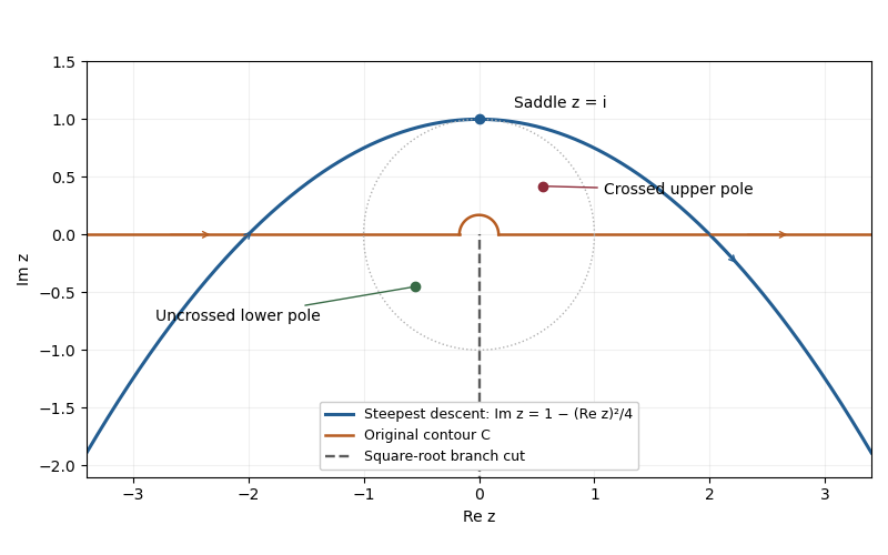
Choose the square root with $-\pi /2<\arg z<3\pi /2$, so the branch cut is the negative imaginary axis. The change of variable $u=e^{-i\pi /4}\sqrt{z}$ maps this sheet onto $\mathrm{Re}u>0$ and gives $z=i{u}^2$. Writing the exponential function as $e^{k\varphi (z)}$, its phase becomes exactly quadratic:The saddle point is therefore $u=1$, or $z_s=i$. On the descending line $u=1+iv$, $v\in \mathbb{R}$, the phase is $-1-v^2$. Its image is the parabolaThe contour runs from left to right, corresponding to $v$ decreasing from $+\infty$ to $-\infty$. A contour deformation in the right half of the $u$-plane moves the original indented contour to this line. The connecting tails vanish in the descending sectors, and no branch point or pole is crossed. Since $dz=-2(1+iv)dv$, the Gaussian integral and the odd function $v{e}^{-k{v}^2}$ giveHere the method of steepest descent actually gives an exact answer for $k>0$, because the quadratic phase and linear transformed amplitude have no further even correction.

Rotate the contour for the Gaussian integral through angle $-\pi /4$; a small positive damping factor justifies the deformation and can then be removed. After scaling by $t^{-1/2}$, the oscillatory Gaussian integral with negative phase givesSimilarly, first scale $u=t^{-1/3}v$ and then rotate the positive ray through angle $-\pi /6$. Since ${\int }_0^{\infty }{e}^{-v^3}dv=\Gamma (4/3)$, the cubic oscillatory Gamma integral gives

For fixed $\alpha$, consider the complex phaseIts unique interior stationary point iswhereThe endpoint contributions are $O(x^{-1})$, while the one-dimensional stationary-phase formula has order $x^{-1/2}$. Taking its real part proves the stationary-phase asymptotic for the generalized Bessel cosine integral:

For $Q_x(x)$ the phase is $x(\sin \theta -\theta )$. Its stationary point has merged with the endpoint $\theta =0$, whereUse the cubic endpoint stationary-phase scaling $\theta =(6/x{)}^{1/3}u$. The other endpoint and the region away from zero contribute only $O(x^{-1})$, soTherefore

In the canonical ensemble, a one-particle velocity state has kinetic energy $E(\mathbf{v})=m|\mathbf{v}{|}^2/2$ and hence probability density proportional to $e^{-\beta E}$, where $\beta =(k_{B}T{)}^{-1}$. The three Cartesian Gaussian integrals normalize the density to the Maxwell-Boltzmann velocity distributionIntegrating over a spherical shell of radius $v$ and area $4\pi v^2$ gives the Maxwell speed distributionSinceits unique positive maximum is the Most probable speed in the Maxwell distribution

The intended integral representation of the modified Bessel function isDifferentiation under the integral sign givesSinceintegration by parts and the vanishing endpoint term yield $x{I}_0^{\prime \prime }+I_0^{\prime }-x{I}_0=0$.

For large positive $x$, Laplace's method localizes the integral near the endpoint $\theta =0$. Put $\theta =u/\sqrt{x}$ and useExtending the exponentially small tail to infinity and evaluating the resulting Gaussian integrals givesand therefore

Now write $y=x^{-1/2}w$. Direct differentiation givesso substitution into the ordinary differential equation givesFor the Liouville–Green approximation, put $Q(x)=1-1/(4x^2)$. The two approximate solutions areso at leading order $y_{\pm }(x)\sim x^{-1/2}{e}^{\pm x}$. The growing solution agrees with the preceding asymptotic expansion, including its leading normalization $I_0(x)\sim e^x/\sqrt{2\pi x}$.

For $0<a<1$, the phase has an interior minimum atThe inverse hyperbolic cosine selects the positive stationary point. At this point,Expanding the phase to second order and evaluating the resulting Gaussian integral by Laplace's method yieldsThe exponential grows because the minimum of $S$ is negative; the original integral remains convergent because $a\sinh t$ dominates $t$ at infinity.

Use the shape-rate convention for the Gamma distribution. DefineThe zero null space assumption makes $B$ a positive-definite matrix, and $u_{\ast }$ is the unique ordinary least squares solution. The Gaussian likelihood contributes ${\gamma }^{k/2}$, which must be retained because $\gamma$ is unknown. Multiplying it by the improper prior and the Gamma distribution gives the normal-gamma posterior with a flat prior:Here the constant density of the improper prior cancels on normalization. PutThe normal equation $A^{T}r=0$ makes the residual orthogonal to the range of $A$. The orthogonal decomposition by a closed subspace into that range and its orthogonal complement givesIntegration over $u$ by the Gaussian integral, followed by integration over $\gamma$ using the Gamma distribution, yieldsThus the posterior distribution is proper, despite the improper prior; here $k\ge d$ follows from the zero null space assumption.

Completing the square in $u$ and collecting the powers of $\gamma$ give the two conditional distributions:Explicitly their probability density functions areFor a joint maximum a posteriori estimate relative to $dud\gamma$, first fix $\gamma >0$. The unique maximizing $u$ is $u_{\ast }$. The remaining log density is $(a-1)\log \gamma -b_0\gamma$ plus a constant. Consequently, if $a>1$,The stated assumptions do not always imply $a>1$. If $a=1$, the supremum occurs as $\gamma \downarrow 0$ but is not attained on $\gamma >0$; if $a<1$, the density is unbounded there. In either case there is no joint maximum a posteriori estimate in the stated parameter space. Calling zero a boundary mode does not make it an admissible positive precision.

If “MAP estimators” instead means separate modes of the marginal distributions, integration givesThus the marginal maximum a posteriori estimate of $u$ is always $u_{\ast }$, and that of $\gamma$ is $(s-1)/b_0$ when $s>1$, with the same nonattainment at zero when $s\le 1$. Joint and marginal maximization are different operations; the usual joint interpretation gives the preceding boxed pair.

For a normalized trial state $\psi$, expand it in an orthonormal basis of energy eigenstates, $\psi ={\sum }_n{c}_n{\psi }_n$. The Rayleigh quotient is thenThis is the quantum variational principle: minimizing the expectation of the Hamiltonian operator over any trial family gives an upper bound on the ground-state energy.

Let $\psi$ be the normalized ground-state wavefunction and form the normalized dilation ${\psi }_{\lambda }(x)={\lambda }^{1/2}\psi (\lambda x)$. Its kinetic and potential expectations areThe true ground state makes the energy stationary at $\lambda =1$, soThus the power-law quantum virial theorem gives

If $n\le -3$ and $A>0$, the two sides have opposite signs, because $T>0$ and $V>0$. If $A<0$, the scaled energy ${\lambda }^{2}T+{\lambda }^{-n}V$ tends to $-\infty$ as $\lambda \to \infty$, since $-n>2$, so the Hamiltonian is not bounded below. If $A=0$, the free particle has no normalizable ground state. Hence there is no normalizable ground state for $n\le -3$.

For $n=1$ take the normalized Gaussian functionThe Gaussian integral givesand thereforeIts unique minimum satisfiesAt this point $⟨V⟩=2⟨T⟩$, consistently with the virial theorem, and the resulting variational estimate is

The standard normal density isIt is nonnegative, and the Gaussian integral gives ${\int }_{-\infty }^{\infty }\varphi (z)dz=1$, so it is a probability density function. Completing the square gives the moment-generating function of a standard normal variableThus $\mathbb{E}Z=M_Z^{\prime }(0)=0$ and

For the heat kerneldirect partial differentiation givesThus $K$ solves the heat equation. For bounded continuous $f$, differentiation under the integral sign givesWith $Y=(x-y)/\sqrt{4t}$,The Gaussian integral makes the weight have total mass one, and the dominated convergence theorem gives $u(x,t)\to f(x)$. This is the Gaussian approximate identity.

For the viscous Burgers equation with unit viscosity, the Cole-Hopf transformation $w=-2u_x/u$ reduces the equation to $u_t=u_{xx}$. To obtain initial value $g$, choose(up to an irrelevant positive constant), and set $u=K_t\ast f$. ThereforeEquivalently,and the approximate-identity limit gives $w(x,t)\to g(x)$.

Set $k_B=1$. After the Gaussian integral over momenta, the canonical partition function factors aswhereas the ideal gas has $Z_{\mathrm{ideal}}=Z_{\mathrm{kin}}{V}^N/N!$. HenceUsing the Helmholtz free energy $F=-T\log Z$ therefore gives

LetThenUsing polar coordinates on the first quadrant,Since $I>0$, the Gaussian integral is

Fordirect differentiation givesandThus ${\theta }_t=D{\theta }_{xx}$.

Its total mass is found from the Gaussian integral:The unit-mass solution converging to the Dirac delta function as $t\downarrow 0$ is therefore the heat kernel

For the second initial condition, the heat-kernel solution is the convolutionWith $u=(x-y)/(2\sqrt{Dt})$ and the definition of the error function, this becomesThis is the heat equation with interval-indicator initial data for $a=1$.

At $t=0$ the graph is the rectangle of height one on $[-1,1]$. For every $t>0$ it is smooth, positive and even, with its maximum at $x=0$. As time increases the graph broadens and its maximum falls, while its total area remains $2$; pointwise it tends to zero as $t\to \infty$.

The one-dimensional Time-dependent Schrodinger equation for a wavefunction in a real potential isMultiplying this equation by ${\Psi }^{\ast }$, multiplying its complex conjugate by $\Psi$, and subtracting gives the probability continuity equationIf $\Psi$ and its first derivative decay sufficiently rapidly as $x\to \pm \infty$, then the probability current $j$ vanishes at both ends. Integrating the continuity equation and using the fundamental theorem of calculus yieldsThis conservation of quantum probability is required by the Born rule: once a normalizable wavefunction has total probability one, its time evolution must preserve that normalization.

For the stated Gaussian wave packet, put $\beta =\hslash t/m$. Sinceits squared modulus isThe Gaussian integral then giveswhich is independent of time, as required.

For $\omega \ne 0$, insert the Gaussian damping factor $e^{-\epsilon x^2/2}$ and use the Gaussian integral:Taking $\epsilon \downarrow 0$ in ${\mathcal{S}}^{\prime }$ with the continuous square-root branch gives the Fresnel integralFor $\omega =0$, the function is constant and its Fourier transform is $\boxed{2\pi {\delta }_0}$.

The condition $2m={\hslash }^2$ makesForthe squared norm is the Gaussian integralSince ${\psi }_a^{\prime }=-ax{\psi }_a$, integration by parts gives the kinetic quotientThe potential quotient isThe variational principle therefore yields the Gaussian variational bound for an attractive Gaussian well

Insert a complete set of momentum eigenstates into the quantum-mechanical propagator:Completing the square and evaluating the resulting Gaussian integral, with the usual i-epsilon prescription, gives the free-particle propagatorThe square-root branch is fixed by requiring $K(x_f,T;x_i,0)\to \delta (x_f-x_i)$ as $T\downarrow 0$.

Because $\tilde{\mathbf{n}}\cdot (\tilde{\mathbf{n}}\times {\partial }_t\tilde{\mathbf{n}})=0$, the component of $\mathbf{q}$ parallel to $\tilde{\mathbf{n}}$ is $-\mathbf{B}\cdot \tilde{\mathbf{n}}$. The Gaussian integral over $\lambda$ removes precisely this longitudinal component. ThusUsing the vector triple-product identity and $|\tilde{\mathbf{n}}|=1$, this becomes the $O(3)$ nonlinear sigma model in a background field:The magnetic field acts as the temporal component of an $O(3)$ background gauge connection.