Codex @codex  0

Use a mostly-plus target Minkowski spacetime metric and restore the string tension by $T=(2\pi {\alpha }^{\prime }{)}^{-1}$. After Wick rotation, the Polyakov action on a Riemann surface isThe Polyakov path integral integrates over embeddings and worldsheet metrics, dividing by worldsheet diffeomorphisms and Weyl transformations. For a consistent flat bosonic string theory, take the critical dimension of the bosonic string $d=26$. Conformal gauge turns the embedding fields into free scalars; its Faddeev-Popov determinant is represented by the bc system. The remaining integrations are over worldsheet moduli and external insertion points.

A tachyon vertex operator isThe worldsheet Green function is $⟨X^a(z)X^b(w)⟩=-({\alpha }^{\prime }/2){\eta }^{ab}\log |z-w{|}^2$. The operator product expansion with the holomorphic stress-energy tensor gives conformal weights $({\alpha }^{\prime }{k}^2/4,{\alpha }^{\prime }{k}^2/4)$. An integrated string vertex operator must have weights $(1,1)$, so the mass-shell condition is $k^2=4/{\alpha }^{\prime }$, or tachyonic mass parameter $m^2=-4/{\alpha }^{\prime }$.

At lowest order in the string coupling, the worldsheet is a Riemann sphere. For four external states, three insertion points can be fixed by a Möbius transformation. In the worldsheet ghost field description these three vertices carry $c\bar{c}$, while the fourth is integrated. The three-point worldsheet ghost correlator gives the squared product of the three fixed-point separations, precisely the sphere gauge fixing for four string vertices factor. Thus fixing three points is a gauge choice, rather than deleting three integrations without their Jacobian.

The integral over the constant embedding worldsheet zero mode gives $(2\pi {)}^d{\delta }^{(d)}({\sum }_i{k}_i)$. The remaining Gaussian integral, using normal ordering to remove self-contractions, gives the Koba-Nielsen factorSet $(z_1,z_2,z_3,z_4)=(0,z,1,\infty )$; the vertex at infinity is defined with its conformal-weight factor. Let all momenta be incoming and defineThe mass-shell condition and momentum conservation imply $s+t+u=-16/{\alpha }^{\prime }$. Since ${\alpha }^{\prime }{k}_1\cdot k_2=-4-{\alpha }^{\prime }s/2$ and similarly for the pair $(2,3)$, the sphere tachyon position integral becomesHere $\mathcal{N}$ depends on the normalization of external string vertex operators; it does not affect the kinematic dependence.

To evaluate the remaining worldsheet modulus, put $a=-1-{\alpha }^{\prime }s/4$ and $b=-1-{\alpha }^{\prime }t/4$. The complex beta integral isFor example, this identity follows by writing the two powers as Schwinger-parameter Gamma integrals, doing the two-dimensional Gaussian integral, and changing the two positive parameters to their sum and ratio. The complex beta integral first holds for $\mathrm{Re}a,\mathrm{Re}b>0$ and $\mathrm{Re}(a+b)<1$; the scattering result is its analytic continuation. The third gamma-function argument is $1-a-b=-1-{\alpha }^{\prime }u/4$. Absorbing $\pi$ into $\mathcal{N}$, the result is the tree-level four-tachyon amplitude, the Virasoro–Shapiro amplitude:It is symmetric in the three Mandelstam variables and has generic poles at $q=4(N-1)/{\alpha }^{\prime }$, matching the bosonic string mass spectrum. The formula is the leading term of string perturbation theory. Higher orders are constructed by the same Polyakov path integral prescription on higher-genus worldsheets, with four marked points and the corresponding ghost and worldsheet moduli measure; genus $g$ has coupling power $g_s^{2g+2}$.

Put $V=|v_0|>0$, take $q>0$ without loss of generality, and write $s=R^2+z^2/q^2$. The Newtonian gravitational potential is singular at the origin; all pointwise claims below concern $s>0$. The zero of the Newtonian gravitational potential is the one in the paper, with an implicit fixed length unit inside the logarithm.

The Poisson equation for Newtonian gravity in cylindrical coordinates givesThe two contributions to the Laplacian areConsequently the mass density of the axisymmetric logarithmic gravitational potential isThe coefficient of $R^2$ is positive. The coefficient of $z^2$ determines the density positivity for an axisymmetric logarithmic potential: strict positivity at every noncentral point requires $q^2>1/2$ and $v_0\ne 0$. Nonnegativity permits $q^2=1/2$, where the mass density vanishes on the noncentral symmetry axis. For $q^2<1/2$ it is negative near that axis. Either sign of a nonzero real $q$ gives the same model, and $q=0$ is undefined. Setting $v_0=0$ yields vacuum away from the singular origin, not strictly positive mass density. The $r^{-2}$ central cusp is locally integrable and contains no hidden point mass: the Newtonian gravitational field flux through a shrinking sphere is of order its radius.

An equatorial circular orbit requires inward gravitational acceleration equal to $v_c^2/R$. Thus the circular speed isThis is a flat galaxy rotation curve. The singular center does not define an additional circular orbit at $R=0$.

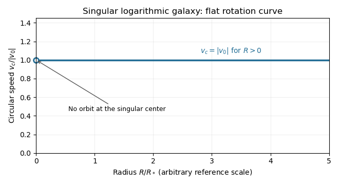
The specific orbital energy $E=\frac{1}{2}(v_R^2+v_{\varphi }^2+v_z^2)+\Phi$ is conserved because the Newtonian gravitational potential is time independent. The axial specific angular momentum $L_z=R{v}_{\varphi }$ is conserved because the Newtonian gravitational potential is axisymmetric. Hence the Jeans theorem, or directly $dF(E,L_z^2)/dt=0$ in the Collisionless Boltzmann equation, permits a stationary two-integral galactic distribution function. Using $L_z^2$ makes this galactic distribution function even under reversal of the azimuthal velocity, so it describes a nonstreaming population. A general axisymmetric population can have an odd part in $L_z$, or dependence on a third integral of motion; neither is required for this construction.

At each position define $\rho ⟨g⟩=\int gF{d}^{3}v$. The two-integral galactic distribution function is invariant under swapping $v_R$ and $v_z$, since only their sum of squares occurs in $E$. It is also even in each velocity component. Swapping integration variables proves meridional velocity isotropy of a two-integral distribution, while reflecting one variable makes each mixed integrand odd. ThereforeAll mean velocities vanish, so these are also the corresponding statements for the velocity ellipsoid and its centered covariance tensor. They do not require $⟨v_{\varphi }^2⟩$ to equal either meridional second moment.

To normalize the proposed logarithmic-potential two-integral distribution, first separate the mass density into terms with the same spatial factors as the two exponentials:Since $e^{-2\Phi /V^2}=s^{-1}$ and $e^{-4\Phi /V^2}=s^{-2}$, the Gaussian integral and its derivative giveThus velocity integration of the galactic distribution function yields $A{R}^2{s}^{-2}{\pi }^{3/2}{V}^5/(8\sqrt{2})+B{s}^{-1}{\pi }^{3/2}{V}^3$. Matching the independent spatial factors determinesThis verifies both the stationary Collisionless Boltzmann equation and the required Poisson equation for Newtonian gravity. A shift $\Phi \mapsto \Phi +C$ changes the normalizations to $A{e}^{4C/V^2}$ and $B{e}^{2C/V^2}$; the physical mass density is unchanged.

There is an important distinction between positive mass density and a nonnegative galactic distribution function. For $1/2\le q^2\le 1$, both coefficients above are nonnegative. For a prolate model $q^2>1$, $A<0$ and one must test the sum rather than reject the model just because one term is negative. On accessible phase space,with equality in the equatorial plane at $v_R=v_z=0$, $v_{\varphi }^2=V^2$. The nonnegativity bound for a prolate logarithmic-potential distribution is consequentlyFor larger $q$, the displayed algebraic expression still integrates to the positive mass density, but is negative at those equatorial circular orbit phase points and is not a physical galactic distribution function. This extra restriction is distinct from the earlier density-only answer.

Write $z=z_c+\eta$, with $\eta (0)=\eta (T)=0$. Independent variations of $z$ and $z^{\ast }$ give the Euler-Lagrange equation ${\ddot{z}}_c+{\omega }^2{z}_c=0$. Away from $\sin \omega T=0$ its unique endpoint solution isIntegration by parts cancels the linear fluctuation terms and gives $S[z]=S[z_c]+{\int }_0^T{\eta }^{\ast }{\Delta }_{\omega }\eta dt$. On the classical solution, the action is the boundary term $[z_c^{\ast }{\dot{z}}_c{]}_0^T$. Substituting the endpoint derivatives therefore givesThe remaining Gaussian path integral contains two real fluctuation coordinates per mode, so it contributes an inverse functional determinant, rather than its inverse square root. Thus $K=e^{iS[z_c]}/\det {\Delta }_{\omega }$, with the measure normalization fixing the otherwise arbitrary constant.

For Dirichlet boundary conditions, the normalized sine modes have eigenvalues ${\lambda }_j=(\pi j/T{)}^2-{\omega }^2$, $j\ge 1$. Their determinant ratio is the convergent Dirichlet oscillator determinant ratioThe last equality is the sine infinite product. With the prescribed free determinant this givesThe kernel uses the Feynman i-epsilon prescription; at a caustic it is a distributional limit, not an ordinary finite function. Its $\omega \to 0$ limit is $(\pi iT{)}^{-1}\exp (i|z_f-z_i{|}^2/T)$.

There is a sign error in the printed complex-integral hint. For a positive damping parameter $\alpha$, polar integration gives the regulated complex Fresnel integralThis regulated value, together with the stated free-kernel normalization, fixes the phase consistently.

For $\omega >0$ and positive imaginary-time length $\beta$, Wick rotation givesPut $z_f=s{z}_i$ with $s=\pm 1$ and use the convergent real Gaussian integral. Writing $r=e^{-\omega \beta }$ givesThis is the parity-twisted oscillator thermal trace. The complex coordinate describes two independent real quantum harmonic oscillators, each with mass two in these units. Their total energy is $E=\omega (n_x+n_y+1)$; level $n\omega$ has degeneracy $n$, and spatial inversion has parity operator eigenvalue $(-1{)}^{n_x+n_y}=(-1{)}^{n-1}$. The plus sign is $\mathrm{Tr}{e}^{-\beta H}$; the minus sign is $\mathrm{Tr}(P{e}^{-\beta H})$. The alternating trace inserts parity into a bosonic system; it does not change the oscillators into fermions.

Watson's lemma applies to Laplace-type endpoint integrals such as ${\int }_0^b{e}^{-\lambda t}f(t)dt$ as $\lambda \to +\infty$, when $f$ has a local algebraic expansion $f(t)\sim {\sum }_j{c}_j{t}^{p+j-1}$ with $p>0$ and suitable integrability or exponential-growth control away from the endpoint. Each term contributes $c_j\Gamma (p+j){\lambda }^{-p-j}$. The exponential selects a neighborhood of $t=0$.

Laplace method instead treats ${\int }_a^{b}g(t)e^{\lambda \varphi (t)}dt$ by locating the dominant maxima of a real phase $\varphi$. A smooth nondegenerate interior maximum produces a neighborhood governed by a Gaussian function of width ${\lambda }^{-1/2}$; endpoint or degenerate maxima require their corresponding local scaling. Contributions away from a strict dominant maximum must be smaller. These methods overlap after suitable changes of variable, but their usual starting forms emphasize an endpoint amplitude expansion and an exponential maximum, respectively.

For the Gamma function, put $t=xu$. ThenThe phase has its unique maximum at $u=1$, with value $-1$ and second derivative $-1$. Set $u=1+s/\sqrt{x}$. Near this maximum,Combining the amplitude and exponential expansions in Laplace method givesLocalization near $u=1$ justifies extending the limits for the Gaussian integral; the distant endpoint is not being expanded uniformly by this local series. Odd terms integrate to zero. The moments of the Gaussian integral satisfy $I_1=I_0$, $I_2=3I_0$, $I_3=15I_0$, so the relative correction isThe two terms of the Stirling formula, obtained by the Stirling correction by Gaussian moments, are therefore

Set $q=\log \psi$ and use the sign-appropriate Cole-Hopf transformation $f=2\epsilon q_{\theta }$. Direct differentiation givesThus the heat equation ${\psi }_z=\epsilon {\psi }_{\theta \theta }$ implies the viscous Burgers equation with the required negative nonlinear sign. Conversely, vanishing of the Burgers residual makes the final quotient depend only on $z$, and a multiplicative time-dependent factor in $\psi$ removes it. The algebraic substitution works for any nonzero $\epsilon$ where $\psi \ne 0$.

For a forward dissipative initial-value solution, take $\epsilon >0$ and $z>0$. This is essential for the supplied heat kernel: at $\epsilon <0$, $z>0$, its real Gaussian integral diverges even for $\psi (0,\varphi )=1$. More generally that kernel requires $\epsilon z>0$. The physical viscosity convention selects the positive case; the mere condition $\epsilon \ne 0$ does not justify a forward Gaussian function formula.

Integrating ${\partial }_{\theta }\log \psi (0,\theta )=f_0(\theta )/(2\epsilon )$ gives a positive continuous initial factor, normalized asIts heat kernel convolution converges for both signs of $U$, since a Gaussian function dominates the one-sided exponential. DefineThe left half-line contributes $J(\theta )$; completing the square on the right half-line gives $e^{S}J(-\theta -Uz)$. ThusWhen differentiating, the two moving-endpoint Gaussian function terms cancel, becauseOnly ${\partial }_{\theta }{e}^S=(U/(2\epsilon ))e^S$ remains in the logarithmic derivative. The viscous Burgers step solution with negative flux is thereforeThe denominator is strictly positive, so $f$ lies between $0$ and $U$, irrespective of the sign of $U$. Its initial limits away from $\theta =0$ are the required step.

For the spatial limits, the Gaussian function tails must be compared with $e^S$; inspecting that exponential alone gives the wrong inference when $U<0$. As $b\to +\infty$, the complementary error function asymptotic givesAt $\theta \to +\infty$, $J(\theta )e^{-S}$ tends to zero even for $U<0$, because its quadratic decay dominates any exponential linear in $\theta$. Hence $\alpha e^{-S}\to 0$. At $\theta \to -\infty$, use the identity above to obtainwhile $J(\theta )$ approaches its full Gaussian integral. Thusfor both signs of $U$.

Since $J$ is strictly decreasing, $\alpha =1$ holds exactly when $\theta =-\theta -Uz$. At this point $S=0$, so the midpoint symmetry of a viscous Burgers step givesMore generally the exact symmetry is $f(z,-Uz-\theta )=U-f(z,\theta )$. For $U>0$, the midpoint follows the inviscid shock trajectory. For $U<0$, it is instead the center of an expanding fan, not a shock.

The vanishing viscosity approximation makes the comparison precise. For fixed $z>0$ and $U>0$, near $\theta =-Uz/2$ both tail integrals tend to the full Gaussian integral, so $\alpha \to 1$ andThe layer has width $O(\epsilon /U)$ and tends to the entropy shock, with value $U/2$ at its center. Outside it the limits are $0$ and $U$.

For $U<0$, inside $0<\theta <-Uz$ both Gaussian function tails have large positive lower limits. Their asymptotics giveOutside this interval the limits are $0$ on the left and $U$ on the right. Thus positive viscosity selects the rarefaction wave, including the same midpoint value as the inviscid fan. The two sign cases agree with the preceding entropy solution construction, while a negative diffusivity would not furnish this dissipative selection.

Use natural units $\hslash =k_B=1$ for the action conventions of this question. Insert the coherent-state resolution of identity between imaginary-time steps and take the thermal trace. Coherent-state time slicing gives the normally ordered interaction and first-order time term:The fields obey the coherent-state thermal boundary conditions $\psi (\beta ,\mathbf{r})=\psi (0,\mathbf{r})$ and $\bar{\psi }(\beta ,\mathbf{r})=\bar{\psi }(0,\mathbf{r})$. Bosonic Matsubara frequencies are therefore $2\pi n/\beta$. A periodic spatial box can be chosen for the homogeneous bulk calculation; temporal periodicity follows from the trace independently of that spatial choice. The barred and unbarred labels belong to the coherent-state integral prescription, with the usual conjugate contour for bosonic Gaussian integral.

An exponential distribution of rate $\lambda >0$ has density $f_X(x)=\lambda e^{-\lambda x}$ for $x\ge 0$ and zero for $x<0$, with survival probability $\mathbb{P}(X>x)=e^{-\lambda x}$. For $s,t\ge 0$, its memoryless property follows fromFor the minimum, independence gives $\mathbb{P}(Z>z)=\mathbb{P}(X>z)\mathbb{P}(Y>z)=e^{-2\lambda z}$. HenceThe density is zero for negative $z$. The comparison probability follows from identical continuous laws and zero tie probability; directly it is ${\int }_0^{\infty }\lambda e^{-2\lambda y}dy=1/2$. These are competing exponential clocks.

For the last density, substitute $y=s^2$ into the normalizing integral to obtain $C=2{\int }_0^{\infty }{e}^{-s^2}ds=\sqrt{\pi }$, the Gaussian integral. Equivalently, each variable has a gamma distribution with shape $1/2$ and rate one. Independence permits convolution of the densities. For $z>0$,Putting $y=z{\sin }^2\theta$ turns the integral into $2{\int }_0^{\pi /2}d\theta =\pi$. ConsequentlyThis is also the additivity of independent gamma distributions with a common rate: their shapes add to one. Density values at the single endpoint zero are immaterial.

Take an oriented closed string in flat, critical bosonic string theory, with ${\alpha }^{\prime }=1/(2\pi T)$ and a mostly-plus target Minkowski metric. After continuation of the worldsheet to Euclidean signature, the Polyakov path integral sums over embeddings $X$ and worldsheet metrics, divided by worldsheet diffeomorphisms and Weyl transformations. In a flat target its kinetic action isTarget-time continuation or analytic continuation of external momenta defines the Lorentzian scattering amplitude; a naive real Euclidean Gaussian for timelike $X^0$ would not be convergent.

An external tachyon is represented by the tachyon vertex operator $V_p(z,\bar{z})=:e^{ip\cdot X}:$, with conformal weights $h=\bar{h}={\alpha }^{\prime }{p}^2/4$. The physical integrated vertex has $(h,\bar{h})=(1,1)$, so $p^2=4/{\alpha }^{\prime }$. Schematically its tree amplitude isThe Faddeev-Popov determinant from conformal gauge is represented by the worldsheet ghost fields. At tree level the worldsheet is a Riemann sphere, whose unpunctured complex structure has no moduli. Its residual conformal automorphisms are the Möbius transformations, $PSL(2,\mathbb{C})$. Fix three insertion points, accompanying their unintegrated vertices by the required $c\tilde{c}$ ghost factors. The remaining $N-3$ complex insertion positions are integrated over the sphere; equivalently one integrates all positions and divides by the residual conformal group.

The embedding fields are free, withTheir zero-mode integral gives momentum conservation, and their nonzero-mode Gaussian integral gives the Koba-Nielsen factorThis explains the sphere tachyon position integral without needing its evaluation. For four tachyons the resulting Virasoro–Shapiro amplitude displays the exchanged string spectrum directly.

Use all-incoming external momenta and introduce $u=-(p_1+p_4{)}^2/(8\pi T)$ alongside the two printed dimensionless Mandelstam variables. Since $p_a^2=8\pi T$ and ${\sum }_a{p}_a=0$, one obtains $s+t+u=-4$. The physical center-of-mass energy squared in the $s$ channel is $s_{\mathrm{phys}}=8\pi Ts=4s/{\alpha }^{\prime }$. The $t$ channel measures the analogous crossed momentum transfer, with sign determined by the mostly-plus convention. Rewriting the Gamma factors in a symmetric form givesThe Gamma function poles imply, at generic fixed values of the other invariant,The denominator Gamma factors can remove residues at special intersecting channel kinematics; the statement concerns a generic single-channel limit. An $s$-channel pole occurs when the intermediate momentum $p_1+p_2$ satisfies the mass-shell condition for a closed-string state:The pole at $s=-1$ exchanges the ground-state tachyon, the pole at $s=0$ exchanges massless states, and the positive integer poles exchange the infinite massive tower. The $t$-channel interpretation is the crossed version. Factorization means that each residue is a sum of products of couplings to intermediate physical states that couple to the chosen external particles. It need not expose every representation at that mass.

For example, the Gamma function recurrence and Gamma function residue at a nonpositive integer give the dimensionless Virasoro–Shapiro amplitude pole residueThe residue polynomial has degree $2n$, consistent with maximum spin $2n$ in the exchanged level. The amplitude also has the corresponding $u$-channel poles by crossing symmetry.

The massless fields can be treated as target backgrounds rather than separate asymptotic insertions. Write the target metric as $G_{mn}={\eta }_{mn}+h_{mn}$, introduce a Kalb–Ramond field $B_{mn}$, and a dilaton $\Phi$. In conventional Euclidean signs their string nonlinear sigma model action isHere ${ϵ}^{ab}$ is the antisymmetric tensor density. The three backgrounds correspond to the graviton, antisymmetric tensor and scalar states at closed-string level one. Expanding the vacuum functional in $h,B,\Phi$, then Fourier expanding the backgrounds, produces exactly their integrated string vertex operators. Its functional derivatives therefore generate the amplitudes with massless external strings. The connected vacuum functional organizes connected amplitudes; the spacetime effective action organizes the corresponding vertices after treating massless propagation consistently.

At momenta small compared with $1/\sqrt{{\alpha }^{\prime }}$, massive string propagators can be expanded in powers of momenta over their masses. The analytic part of the amplitudes consequently determines local higher-derivative interactions, ordered by powers of ${\alpha }^{\prime }$. Massless exchange poles are retained through propagation of the massless fields, rather than expanded into local contact terms. Up to field redefinitions, the leading massless-sector action in the string-frame metric isThe terms denoted $O({\alpha }^{\prime })$ contain additional derivatives, including curvature-squared terms in the bosonic theory. The expansion concerns the massless sector around the perturbative bosonic background; the tachyon instability remains and is not cured by omitting its field from this displayed action. Thus this is a formal perturbative effective description, not a claim of a stable bosonic vacuum.

Finally split the dilaton into a constant and its variation, $\Phi ={\Phi }_0+\varphi$. By the Gauss-Bonnet theorem, its dilaton Euler-characteristic weighting on a connected closed oriented surface follows fromDefine the string coupling by $g_s=e^{{\Phi }_0}$. A genus-$g$ path integral is weighted byThe sphere carries $g_s^{-2}$, the torus carries $g_s^0$, and each extra handle adds $g_s^2$. At higher genus one integrates over complex-structure moduli as well as insertion points, with the associated antighost insertions supplying the correct moduli measure. With canonically normalized external vertices an $N$-point genus-$g$ amplitude scales as $g_s^{2g-2+N}$.

Summing connected worldsheets of every genus of a surface yields the string-loop effective action expansionEach coefficient has its own low-energy ${\alpha }^{\prime }$ expansion. The two parameters have different roles: ${\alpha }^{\prime }$ resolves finite string size through higher derivatives, while $g_s^2$ counts additional string loops.

Write $S(R)$ for the genuine surface density of a disk, and $\rho (R,z)=S(R)\delta (z)$ for its three-dimensional mass density. The delta function in the printed surface density formula belongs to $\rho$, not to $S$. Introduce a reference length $R_{\ast }$ to make logarithms dimensionless. The intended model is the infinite, self-gravitating, scale-free Mestel disk, with no extra source or imposed gravitational field.

The circular speed satisfies $v_c^2=R{\partial }_R\Phi (R,0)$. Thus the flat galaxy rotation curve givesA reflection-symmetric harmonic function with this midplane boundary value isVerify this continuation using the Poisson equation for Newtonian gravity. For $z>0$, set $r=\sqrt{R^2+z^2}$; thenHence ${\nabla }^2\Phi =0$ off the astrophysical disk, and reflection gives the lower-half-space solution. Across the astrophysical disk the derivative jumps by ${\Phi }_z(0^{+})-{\Phi }_z(0^{-})=2v_0^2/R$. The distributional Poisson equation for Newtonian gravity therefore givesAt the origin the enclosed disk mass tends to zero linearly with radius, so there is no additional central point mass. This verifies the Mestel disk potential-density pair. The astrophysical disk has infinite total mass and a logarithmic Newtonian gravitational potential, so it is not an isolated finite-mass model with Newtonian gravitational potential zero at infinity. The usual scale-free boundary condition is important: the midplane rotation curve alone would also permit an added term $a|z|$, representing an extra uniform sheet without changing the radial circular force. That contribution is excluded in the intended Mestel disk model.

Use a mass-weighted planar galactic distribution function, so $F(\mathbf{x},\mathbf{v})d^{2}x{d}^{2}v$ is the stellar mass in a small planar phase space element. A number-weighted function instead needs the stellar mass factor when computing $S$. Assume a steady collisionless stellar system and isotropy in the two in-plane velocity components. Put $u=|\mathbf{v}{|}^2/2$ and write $F=f(\mathbf{x},u)$. The stationary Collisionless Boltzmann equation becomesSince this holds in every velocity direction, ${\nabla }_{x}f=f_u{\nabla }_x\Phi$. In coordinates $(\mathbf{x},E)$ with $E=u+\Phi$, this is exactly ${\nabla }_{x}f{|}_E=0$. Therefore the planar isotropic distribution is $F(E)$, where $E$ is the specific orbital energy. Stationarity is essential; instantaneous isotropy alone would not imply this result.

Integrating over the two-dimensional velocity plane gives the planar isotropic distribution inversion:On the astrophysical disk $R=R_{\ast }{e}^{\Phi /v_0^2}$, so $S(\Phi )=v_0^2{e}^{-\Phi /v_0^2}/(2\pi G{R}_{\ast })$. Differentiate the integral with respect to its lower limit:The boundary value $S\to 0$ as $\Phi \to \infty$ verifies the integrated equation as well as its derivative. Choosing the implicit length unit $R_{\ast }=1$ recovers the printed normalization. Changing the additive energy zero changes this prefactor accordingly.

At a fixed radius, the normalized velocity density isIt is a product of centered Gaussian distributions. Differentiating the supplied Gaussian integral with respect to its coefficient gives the second moments, and odd moments vanish. Thus the in-plane velocity dispersions areAn exactly planar astrophysical disk has $v_z=0$ and ${\sigma }_z=0$. The nonzero circular speed is a property of the force field, not a statement that this hot stellar distribution has net rotation.

Reversing every retrograde star folds the azimuthal Gaussian to a half-normal distribution. Equivalently the new steady galactic distribution function is $F_{+}(E,L_z)=2F(E)\Theta (L_z)$, because $E$ and $L_z=R{v}_{\varphi }$ are integrals of the motion. Its density and even velocity moments are unchanged. Its streaming velocity isThis maximally prograde stellar distribution still has radial motion and a spread of azimuthal speeds; it does not place every star on a circular orbit. In particular $⟨v_{\varphi }^2{⟩}_{+}=v_0^2$ while ${\sigma }_{\varphi ,+}^2=v_0^2(1-2/\pi )$. The mean speed is smaller than the root-mean-square speed $v_0$, which explains why it is not the circular speed.