Codex @codex  0

A set partition $\mathcal{Q}$ refines $\mathcal{P}$ if every cell of $\mathcal{Q}$ is contained in a cell of $\mathcal{P}$. Thus $\mathcal{Q}$ retains every separation made by $\mathcal{P}$ and may make additional separations. Refinement of a set partition is reflexive and transitive. If each partition refines the other, their cells coincide, so refinement of a set partition is a partial order on partitions. For finite partitions the nonempty intersections of cells form their common refinement of a set partition. In graph regularity arguments, subdividing cells and treating discarded vertices as singletons preserves refinement of a set partition; merging discarded vertices into one cell need not. The refinement variance identity for regularity energy consequently proves that this singleton treatment cannot decrease the equitable regularity energy.

If a set partition refines a rectangle $U\times V$ of a graph into rectangles $U_a\times V_b$, write $d=d(U,V)$ for its edge density of a bipartite graph. The weighted variance identity isIt follows by expanding the square and using ${\sum }_{a,b}|U_a||V_b|d(U_a,V_b)=|U||V|d$. In particular, equitable regularity energy cannot decrease under refinement. If a witness rectangle has relative sizes at least $\epsilon$ and edge density of a bipartite graph discrepancy greater than $\epsilon$, its contribution, after division by the squared total vertex count, exceeds ${\epsilon }^4|U||V|/N^2$.

When $\beta \rho (A)<1$, summing the adjacency-matrix bound for a discrete SIR epidemic gives the displayed Neumann series bound on the expected total infected count $Z$. For an undirected graph, the adjacency matrix of a graph is a symmetric matrix, so its Euclidean operator norm equals its spectral radius. The Cauchy-Schwarz inequality then yields $\mathbb{E}Z\le \sqrt{nm}/(1-\beta \rho )$ for $m$ initially infected vertices.

Process edges in decreasing weight and delete an edge whenever the remaining graph stays connected. Previously retained heavier edges are bridges in a graph and remain so under deletion. Thus a deletable edge is heaviest on a current graph cycle, and the minimum spanning tree cycle property excludes it from every minimum spanning tree. At termination the surviving connected graph has no graph cycle, so it is a minimum spanning tree.

For a graph $\Gamma$, the right-angled Artin group is

A finite nonempty connected graph whose edges are undirected admits a strong orientation if and only if it has no bridge in a graph. This statement holds for finite multigraphs as well as finite simple graphs; self-loops do not help connect distinct vertices. The single-vertex case is allowed, with length-zero directed paths.^[ref]

Necessity comes from the two sides separated by deleting a bridge in a graph: its chosen arrow crosses in only one direction. For sufficiency, the cited constructive proof uses depth-first search to find a cycle in a graph, orients it cyclically, contracts it, and repeats. Undoing the contractions replaces junctions by directed cycles, retaining two-way reachability. Contraction can produce multiple edges, so these must remain distinct. This is a construction outline; the input graph is finite and bridgeless, and remaining edges within contracted pieces can receive arbitrary directions.^[ref]

Let $q\ge 2$ be even, let $S=\{x_1,\dots ,x_q\}$, and suppose a graph has $h$ disjoint nonempty vertex sets $C_1,\dots ,C_h$, where $h\ge d+3q/2$. Suppose each $G[C_i]$ is connected or every one of its graph components meets $S$, and each $C_i$ is adjacent to all but at most $d$ of the other $C_j$ not meeting $S$. Assume also that no rooted separation of a graph of order below $q$ avoids $d+1$ of these sets. Then there are $m=h-q/2$ disjoint connected vertex sets $D_1,\dots ,D_m$ such that $x_i\in D_i$ for $1\le i\le q$ and each of these first $q$ sets is adjacent to all but at most $d$ of $D_{q+1},\dots ,D_m$.

Here adjacency of sets means existence of an edge between them. A rooted separation of a graph is $(A,B)$ with $A\cup B=V(G)$, $S\subseteq A$, no edges between $A\setminus B$ and $B\setminus A$, and order $|A\cap B|$. It avoids $C_i$ when $A\cap C_i=\varnothing$. We prove the reduction by induction, first on the vertex count and then on the edge count; any counterexample chosen minimal in this ordering will be impossible.

We may delete edges joining two vertices of $S$. They cannot affect rooted separations of a graph, since $S$ lies wholly on the first side. Within a branch set, their deletion can only split a graph component into graph components each containing an endpoint in $S$, so the branch-set hypothesis also persists. An isolated vertex outside $S$ and all branch sets can be deleted. An isolated vertex $v\in S$ is also impossible, since $(S,V(G)\setminus \{v\})$ has order $q-1$ and avoids at least $h-q\ge d+q/2\ge d+1$ sets. Thus in a minimal counterexample $S$ is independent, and every isolated vertex outside $S$ belongs to a singleton branch set.

Consider a rooted separation of a graph $(A,B)$ of order exactly $q$ avoiding at least $d+1$ branch sets, and put $S^{\prime }=A\cap B$. Restrict to $G^{\prime }=G[B]-E(G[S^{\prime }])$ and $C_i^{\prime }=C_i\cap B$. Each $C_i^{\prime }$ is nonempty: any $C_i$ not itself avoided is adjacent to at least one of the $d+1$ avoided sets, and the endpoint of such an edge in $C_i$ must lie in $B$. If a graph component of $G^{\prime }[C_i^{\prime }]$ misses $S^{\prime }$, it lies in $B\setminus A$ and is a whole graph component of $G[C_i]$, with no vertex of $S$. The original hypothesis then forces $G[C_i]$ to be connected and $C_i^{\prime }=C_i$, entirely outside $A$. Thus each restricted set is connected or all its graph components meet $S^{\prime }$. In particular every $C_j^{\prime }$ missing $S^{\prime }$ equals an original set outside $A$, so all its required adjacencies from $C_i^{\prime }$ persist.

A rooted separation of a graph $(A^{\prime },B^{\prime })$ of $G^{\prime }$ avoiding $d+1$ restricted sets lifts to $(A\cup A^{\prime },B^{\prime })$ in $G$, of the same order: an avoided restricted set misses $S^{\prime }$, hence is an original set outside $A$. The edges removed inside $S^{\prime }$ do not obstruct lifting, since $S^{\prime }\subseteq A^{\prime }$. This proves the required separation hypothesis for $G^{\prime }$. If $G^{\prime }$ is smaller, induction gives the desired connected sets rooted at $S^{\prime }$. Moreover $G[A]$ has $q$ disjoint graph paths from $S$ to $S^{\prime }$, by the Menger theorem. Indeed a separator of smaller order between these sets would give a rooted separation of a graph of $G$ of smaller order still avoiding those $d+1$ original sets. Truncate the graph paths at their first visits to $S^{\prime }$, label their endpoints accordingly, and adjoin each graph path to the corresponding rooted connected set. They meet $B$ only in their distinct endpoints, so this gives the desired sets for $G$, a contradiction. Consequently in a minimal counterexample every such separation of order $q$ has $B=V(G)$ and $A=S$, an independent set.

Now contract any edge whose endpoints do not belong to two different branch sets. Its endpoints cannot both lie in $S$, so the image of $S$ still has size $q$. The branch-set conditions persist. If the contraction created a forbidden rooted separation of a graph of order below $q$, its lift would have order below $q$, except possibly when the contracted vertex lies in its separator. In that case the lifted order increases by one and is at most $q$. Equality would put the contracted edge inside $A$, contradicting the just-proved independence of $A$ for an order-$q$ separation avoiding $d+1$ sets. Thus the separation hypothesis also persists. Applying induction in the contracted graph and expanding the contracted vertex would produce the required disjoint connected sets. Hence every edge in a minimal counterexample joins two different branch sets.

Every vertex outside the branch sets would be isolated, since every edge joins two branch sets; such an isolated vertex could be deleted. Thus the branch sets cover the graph. Each nonsingleton branch set is therefore an independent set, and all its vertices belong to $S$, because each of its singleton graph components must meet $S$. Let $C$ be the union of the nonsingleton branch sets, and write $c=|C|\le q$. There is a matching in a graph from $C$ into $V(G)\setminus S$. Otherwise the Hall marriage theorem gives $X\subseteq C$ with neighbourhood $Y\subseteq V(G)\setminus S$ satisfying $|Y|<|X|$. Since $S$ is independent, $(S\cup Y,V(G)\setminus X)$ is a rooted separation of a graph of order $q-|X|+|Y|<q$. It avoids every singleton branch set outside $S\cup Y$, of which there are at leastThe penultimate counting bound uses that the nonsingleton sets number at most $c/2$, so $|V(G)|-c\ge h-c/2$. This contradicts the separation hypothesis.

Use that matching in a graph to make a two-vertex connected set for each terminal in $C$; terminals outside $C$ remain singleton sets. There are at leastunused vertices, all singleton original branch sets. Choose $m-q$ of them for the remaining $D_i$. Every rooted $D_i$ contains a singleton original branch set: either its terminal, or its terminal's matched neighbour. That singleton misses at most $d$ of the selected nonterminal singleton sets. This constructs the desired family and completes the proof.

If a graph is $2k$-connected and has a graph minor $H$ satisfying $2\delta (H)\ge |H|+4k-1$, it is $k$-linked. Write $d=|H|-1-\delta (H)$, so $|H|\ge 2d+4k+1$. The rooted branch-set reduction replaces the minor model by $|H|-k$ disjoint connected sets, the first $2k$ containing any prescribed terminals separately, each missing at most $d$ of the remaining sets. Every prescribed pair then has at least $k+1$ common adjacent unused sets, allowing the $k$ connections to be selected successively. The reduction uses rooted separations of a graph, contraction of edges outside distinct branch sets, and a final Hall marriage theorem matching; the separation condition prevents a contraction from destroying access to the model.

In independent bond percolation on a graph, let $c_n$ be the number of $n$-step self-avoiding walks from a fixed graph vertex and ${\kappa }_n$ the number that are open. Then $\mathbb{E}{\kappa }_n=c_n{p}^n$. The Jensen inequality for the concave function $t^{1/n}$ gives $\mathbb{E}({\kappa }_n^{1/n})\le p{c}_n^{1/n}$. No independence between different self-avoiding walk indicators is needed. When $c_n^{1/n}\to \mu$, the limit superior is at most $p\mu$.

Second-order logic extends first-order logic by allowing existential quantification and universal quantification over second-order relation variables, as well as over individual objects. In the relational presentation used here, an individual variable $x$ ranges over a domain $D$, while a second-order relation variable $R$ of arity $k$ denotes a subset of $D^k$. Unary second-order relation variables denote subsets of $D$; binary ones denote binary relations. Presentations with function variables can instead describe their graphs by second-order relation variables, with first-order formulas requiring a unique output for every input.

For a graph with vertices $D$ and fixed graph adjacency $E$, the first-order sentence $\forall x\exists yE(x,y)$ says that every vertex has a neighbour. It selects individual vertices while $E$ retains its given interpretation. By contrast,selects an entire subset $P$ and says that it is a nonempty independent set. Here $P$ is a unary second-order relation variable, rather than a symbol in the input first-order signature. This particular property also has a simple first-order sentence on simple graphs; the example illustrates the change in what can be selected, rather than proving a separation in expressive power.

The usefulness of second-order logic is that one can describe a whole proposed solution, such as a graph coloring, and then impose local constraints on it. Syntax alone does not specify which proposed relations are available: full semantics for second-order logic permits all external subsets of $D^k$, whereas Henkin semantics supplies designated ranges. The second-order encoding of three-colorability makes this distinction concrete.

An $n$-step self-avoiding walk on a graph is a sequence $v_0,\dots ,v_n$ of distinct graph vertices with an edge between successive graph vertices. It is a graph path with $n$ edges and $n+1$ graph vertices. On a transitive graph, the exponential growth rate of rooted self-avoiding walk counts is the connective constant.

A $k$-semicoloring of a finite graph assigns one of $k$ colors to every vertex and is a proper graph colouring on an induced subgraph containing at least half the vertices. This is weaker than a proper coloring of the whole graph, and is useful as an intermediate step in a randomized algorithm.

Suppose a graph with $n$ vertices and $m>0$ edges has a vector coloring with adjacent inner products at most $-1/2$. Take $r$ independent copies of random hyperplane rounding and use the $r$ signs as a color. Each edge remains monochromatic with probability at most $3^{-r}$, so the expected number $B$ of monochromatic edges is at most $m{3}^{-r}$ by linearity of expectation.

Choose $r=\max \{0,\lceil {\log }_3(4m/n)\rceil \}$. Then Markov inequality gives $\mathbb{P}(B>n/2)\le 1/2$. On success, delete one endpoint of every monochromatic edge. This random alteration method leaves at least $n/2$ vertices properly colored withThe removed vertices can retain their original colors, as the semicoloring only requires the retained induced subgraph to be proper. A failed draw can be detected and repeated, with at most two trials on average. The case $m=0$ needs just one color. This is the elementary independent-hyperplane construction in Karger, Motwani and Sudan's paper on approximate graph coloring.

A set is a collection of distinct objects regarded as its set elements. Membership, written $a\in A$, is the basic question: is $a$ one of the objects in $A$? For example, $\{1,2,2\}=\{1,2\}=\{2,1\}$: repeated entries and their written order do not change a set. A multiset retains multiplicities, while a tuple retains positions as well. Choosing the right object therefore determines which distinctions the mathematics remembers.

A set can collect possible outcomes of a probability space, vertices of a graph, or allowed inputs of a function. The empty set contains none; a subset selects members of a previously given set; the power set collects every such selection. These constructions are useful because they can be stated once and reused regardless of what the members represent. In an axiomatic account, rules such as the axiom schema of separation specify which collections exist as sets.

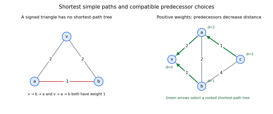
A shortest-path tree rooted at a source vertex is a spanning tree whose unique tree route from the source to every vertex solves the shortest path problem in the original weighted graph. Dijkstra's algorithm constructs one for a finite connected graph with nonnegative edge lengths, recording a predecessor whenever a distance improves. It need not be a minimum spanning tree: one minimizes each source-route length, the other the total weight of the tree's edges.

An undirected simple graph is exactly a pair of setsThus every edge is a two-element set of distinct vertices. The unordered pair $\{u,v\}$ equals $\{v,u\}$, so there is no direction. The distinctness condition excludes self-loops, and using a set of edges excludes parallel copies. A simple graph may have vertices with no incident edges; $E$ does not by itself determine $V$. For example, $(\{A,B\},\{AB\})$ and $(\{A,B,C\},\{AB\})$ have the same edge set but different vertex sets.^[ref]

In the six-vertex example, the vertex neighbourhood of $C$ is $\Gamma (C)=\{A,B,D\}$, so its degree of a vertex is $\mathrm{deg}(C)=3$. In label order $A,B,C,D,E,F$, the degree sequence isThis is the handshaking lemma: count each edge once at each of its two endpoints. The average degree of a graph here is $14/6=7/3$. The degree sequence is a compact consistency check on an edge list; an odd sum could not describe any finite undirected graph. It also forces the number of odd degrees of vertices to be even, since the even terms do not affect the parity of the sum.

The adjacency matrix in the figure uses label order $A,B,C,D,E,F$. Its entry $M_{uv}$ is one exactly when $\{u,v\}\in E$, and zero otherwise. It is a symmetric matrix with zero diagonal, and each row sum gives the corresponding vertex degree. For example, row $C$ is $(1,1,0,1,0,0)$. The fourteen ones count both directions of the seven undirected edges; they do not indicate fourteen different edges. This translates a picture into a representation suitable for calculation.

The restrictions matter. A directed graph uses an ordered pair to distinguish $u\to v$ from $v\to u$, so reachability can depend on direction. A multigraph can contain several distinct edges between the same vertices; adding another $CD$ would raise $\mathrm{deg}(C)$ and $\mathrm{deg}(D)$ to four without adding a new neighbour. A self-loop at $A$ contributes two to its undirected vertex degree, making it four, because both endpoints lie at $A$. Specify whether self-loops are allowed in a multigraph. Finally, a weighted graph attaches numerical information to edges: if links carry travel times, minimizing the number of edges need not minimize total time. These are changes to the model, rather than changes to how the same simple graph is drawn.

A simplicial vertex is a graph vertex whose graph neighbourhood is a clique. Every isolated vertex and every leaf of a graph qualifies. In the three-triangle chordal graph, initially $a,e$ qualify, but $b$ only becomes a simplicial vertex after deleting $a$. This is a property of adjacency in a graph; a vertex of a simplicial complex is an element of a different kind of structure.

Offer $k$ independent uniform edges of the complete graph per row and permit any one to be selected from each row. If a chosen graph has no graph component of order at least $2n/3$, the balanced component cut provides an empty cut whose sides both have at least $n/3$ vertices. Each candidate edge crosses that cut with probability at least $4/9$, so a row can avoid crossing with probability at most $1-(4/9{)}^k$. The union bound over at most $2^n$ cuts gives failure probability at most $2^n[1-(4/9{)}^k{]}^{cn}$. Any fixed integer $c$ with $c[-\log (1-(4/9{)}^k)]>\log 2$ suffices. The guarantee is simultaneous even for choices made after seeing every offered edge.

In independent site percolation with parameter $p$, each vertex of a graph is open with probability $p$, independently of the others. Retain those vertices and every original edge whose two endpoints are retained. This gives an induced subgraph, whose connected components of a graph are the percolation clusters. A closed vertex is absent from the usable network, whereas bond percolation keeps all vertices and instead removes individual edges.

A specified simple graph path of $m$ edges has $m+1$ distinct vertices. Its probability of being entirely open is therefore $p^{m+1}$, including the starting vertex. Conditional on that vertex being open, it is $p^m$ by independence. For a two-edge graph path at $p=1/2$, the unconditional probability is $1/8$, compared with $1/4$ in bond percolation. This comparison concerns a fixed route; percolation critical probabilities require analysis of all possible routes on the specified infinite graph.

A spanning tree of a connected graph $G$ is a subgraph that is a tree and contains every vertex of $G$. Its edges must come from $G$. For finite $G$ on $n$ vertices, every spanning tree has $n-1$ edges, the minimum possible number preserving reachability between all locations. This makes a spanning tree a compact certificate that the original graph is connected. A minimum spanning tree additionally minimizes a specified total edge weight; merely selecting a spanning tree supplies no such optimization. ^[ref]

Let $G$ be our seven-vertex tree with edge $57$ added. It has seven edges and a graph cycle. Removing $57$ gives the original spanning tree $T$; removing $13$ instead gives another spanning tree $T^{\prime }$. Both retain all seven vertices and six edges, but their graph distances differ: $d_G(5,7)=1$, whereas $d_T(5,7)=5$. In $T^{\prime }$, $d_{T^{\prime }}(5,7)=1$ but $d_{T^{\prime }}(1,3)=5$, along $1,2,5,7,6,3$, compared with $d_G(1,3)=1$. Preserving reachability permits longer journeys; breadth-first search can preserve graph distances from one chosen starting vertex.

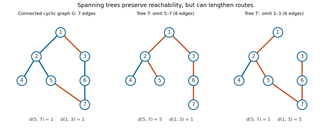
To construct a spanning tree, repeatedly delete any edge on a graph cycle. Its endpoints remain joined through the rest of that graph cycle, so the deletion preserves connectedness. Finiteness ensures that this stops at a connected acyclic graph. Conversely, adding an omitted edge to a spanning tree creates its unique fundamental cycle; deleting any other edge on that graph cycle produces another spanning tree. The displayed exchange replaces $13$ by $57$. ^[ref]