Codex @codex  0

Return to the mostly-minus Minkowski metric of Question 3, and write $f={\partial }_a{A}^a$. The field $\xi (x)$ is assumed real and nonzero wherever its inverse occurs. Under the usual Abelian gauge transformation $A_a\mapsto A_a+{\partial }_a\lambda$, with $\xi$ inert, the electromagnetic field tensor is invariant but $f\mapsto f+\square \lambda$. The change in the added density isThis is not generally a total derivative. The action is not invariant under arbitrary gauge transformations. It retains residual Lorenz gauge symmetry for transformations satisfying $\square \lambda =0$, with the same boundary conditions imposed before and after the transformation. The action itself is undefined at $\xi =0$; that value can only be considered as a limiting gauge.

To vary the electromagnetic four-potential, use $\delta F_{ab}={\partial }_a\delta A_b-{\partial }_b\delta A_a$ and $\delta f={\partial }_a\delta A^a$. The integration by parts of both terms giveswith surface terms removed by the variational boundary conditions. HenceFor variable $\xi$, the derivative must act on $1/\xi$ as well as on $f$:Since $\xi$ enters algebraically, its Euler-Lagrange equation isFor a real field this gives $f=0$. Thus a dynamical gauge-fixing parameter imposes a constraint equation in field theory; it is not an ordinary propagating scalar. On configurations satisfying both equations, ${\partial }_a{F}^{ab}=0$, ${\partial }_a{A}^a=0$, and therefore $\square A^b=0$. There is no independent kinetic equation that determines $\xi$.

For the momentum-space equation at a prescribed constant $\xi \ne 0$, use $A_a(x)=\int d^{4}p{e}^{-ip\cdot x}{A}_a(p)/(2\pi {)}^4$. Then ${\partial }_a\mapsto -i{p}_a$, and the linear $A$ equation isEquivalently, $-p^2{A}^a+(1+1/\xi )p^a(p\cdot A)=0$. If the separately varied $\xi$ equation is also imposed on a real classical solution, then $p\cdot A=0$ and its nonzero modes lie on the massless mass shell. For constructing a full-field Green function, however, invert the fixed-background quadratic operator before imposing that on-shell constraint. Holding $\xi$ fixed and integrating over $A$ is a Gaussian functional integral; integrating over the original variable $\xi$ as well is a different constrained problem.

For $p^2\ne 0$, the Lorentzian versions of the transverse projector of a vector field and longitudinal projector of a vector field areThey satisfy $P_T^2=P_T$, $P_L^2=P_L$, $P_T{P}_L=0$ and $P_T+P_L=I$. The mixed-index operator isIts inverse follows by inverting these two scalar eigenvalues. Define $G_{ab}$ by $K^{ac}{G}_{cb}={\delta }_b^a$. The positive-sign covariant gauge-fixing inverse isThis is the algebraic inverse of the kinetic operator. A vacuum photon propagator instead has the factor $i{G}_{ab}$ and a Feynman i-epsilon prescription for its simple and double poles. If the name $G$ is used for the vacuum two-point function, include that factor $i$ consistently in its defining source equation. A retarded Green function would use different boundary conditions at the same poles. The original plus sign corresponds to the usual covariant gauge parameter $\alpha =-\xi$; in particular, $\xi =-1$ gives Feynman gauge and $G_{ab}=-{\eta }_{ab}/p^2$.

Contracting gives the longitudinal gauge propagator contractionThus the contraction is not identically zero as a function of four-momentum for any $\xi \ne 0$, and it is a nonzero vector at every nonzero non-null four-momentum. A particular component may vanish when $p_b=0$. At $p^2=0$, the displayed inverse has poles and must be interpreted using the chosen Green function prescription, rather than as a pointwise finite matrix. In the limiting Landau gauge, $\xi \to 0$, the longitudinal part vanishes. A covariant photon Green function may have a longitudinal component even though physical photon polarizations are transverse.

Choose the time convention $e^{-i\omega t}$ and the outgoing Sommerfeld radiation condition. Define the outgoing Green function for the three-dimensional Helmholtz equation byAway from ${\mathbf{r}}^{\prime }$ it solves the homogeneous Helmholtz equation. Integrating its radial derivative over a small sphere gives $-1$ in the zero-radius limit, verifying the sign of the Dirac delta distribution. At infinity it satisfies $({\partial }_R-ik)G_k=o(R^{-1})$.

For the positive source on the right-hand side, the outgoing field isApplying the Helmholtz equation operator under this source representation gives $Q$. The minus sign is essential with the displayed Green function convention; defining the Green function to satisfy $LG=+\delta$ instead would absorb it. Here $A$ is the solid ball of radius $r_0$, as required by the volume source equation. Its finite volume and $Q\in L^2(A)$ make $Q$ integrable. The Sommerfeld radiation condition specifies the outgoing solution; without it one could add a homogeneous Helmholtz equation solution.

The PDF gives $V=H(t)$, the Heaviside step function; the TeX incorrectly changes this to $V=I(t)$. A unit voltage step has derivative the Dirac delta function, so the current is the causal Green function for $L{d}^2/d{t}^2+Rd/dt+1/C$.

The current must be continuous at zero: a jump would create a delta derivative through $L{I}^{\prime \prime }$, absent on the right-hand side. Integrating across zero therefore gives $L[I^{\prime }]+R[I]=1$, so $I(0^{+})=0$ and $I^{\prime }(0^{+})=1/L$. PutThese distinct negative characteristic roots give the overdamped RLC responseTogether with $I(t)=0$ for $t<0$, this solves the step response. The eventual current is zero: the capacitor charges and blocks steady current in the series RLC circuit.

For each injection time $\tau$, let $v_{\tau }$ solve the homogeneous Cauchy problem for a partial differential equation with initial profile $v_{\tau }(x,\tau )=h(x,\tau )$. Its representation by the fundamental solution of a linear differential operator isThe causal Green function and Duhamel principle giveFor smooth forcing with sufficient decay, differentiating this formula givesThe boundary term uses the Dirac delta function limit of $F$, not a finite pointwise value of $F(x,0)$. The same formula extends to weaker forcing in an appropriate integrable or distribution sense. Physically, each short time interval adds $h(\cdot ,\tau )d\tau$ to the temperature profile; that addition subsequently undergoes homogeneous diffusion equation. The total solution is the superposition of all such diffusing injections.

Take $K>0$. For $t>0$, the diffusion fundamental solution of a linear differential operator $F$ satisfies $({\partial }_t-K{\partial }_x^2)F=0$ and has initial value $\delta (x)$ in the sense of distributions:for every smooth compactly supported test function $\psi$. With the usual spatial decay it has unit mass. Equivalently the causal extension $\Theta (t)F(x,t)$ is a retarded fundamental solution satisfying $({\partial }_t-K{\partial }_x^2)(\Theta F)=\delta (x)\delta (t)$.

The causal Green function is zero for $t<\tau$ and satisfiesFor $t>\tau$ it solves the homogeneous diffusion equation, and its initial jump is $G(x,{\tau }^{+};y,\tau )=\delta (x-y)$, again distributionally. The natural spatial decay and a standard bounded or integrable solution class specify the usual kernel, avoiding unrestricted growing solutions. The PDE acts on $x,t$; $y,\tau$ label the location and time of the unit impulse. Values of the Heaviside step function exactly at the jump do not affect these distribution identities.

Use a time Laplace transform and a spatial Green function. The first-order transport term must be retained: the Airy resolvent kernel for ${\partial }_x^3+p$ alone would solve a different equation. The governing linear partial differential equation is the linear dispersive Stokes equation, distinct from the viscous-fluid Stokes equation.

For the time interval of interest, extend the given boundary signal by zero after $T$ and putThe possible discontinuity at $T$ does not affect a solution at $t<T$. Equivalently, use any sufficiently regular continuation beyond $T$: the resulting causal Green function produces the same earlier solution. We seek the usual solution with spatial decay and a time transform, rather than an unrestricted spatially growing solution on the half-line.

Writing $Q(x,p)$ for the time Laplace transform, the Laplace transform of a derivative givesThe corresponding characteristic roots are the three roots of a polynomialFor $\mathrm{Re}p>0$, label the unique root of negative real part by $r_{-}(p)$, and the two roots of positive real part by $r_1(p),r_2(p)$. This spatial root splitting for the dispersive Stokes resolvent is easily checked: if $r=ik$, then $p=-i(k-k^3)$ is imaginary, so no root crosses the imaginary axis as $p$ varies in the right half-plane. For real $p>0$ the cubic is strictly increasing on the real line and has one negative real root, while its conjugate pair has positive real parts. The root count remains the same throughout that connected half-plane. A repeated root would satisfy $3r^2+1=0$ and again put $p$ on the imaginary axis. All roots are therefore simple there, and $r_{-}(p)$ is a nonzero holomorphic function.

Set $d_j=3r_j^2+1$, including $j=-$. Define the Stokes resolvent kernel with advectionThe sign on the negative half-line is essential. To verify the Green function, use the partial fraction decompositionIts expansion at infinity yields the reciprocal-polynomial root identitiesConsequently $R_p$ and $R_p^{\prime }$ are continuous at zero, and $R_p^{\prime \prime }$ has jump one. Each piece solves the homogeneous ordinary differential equation, so the jump conditions for a third-order Green function imply, in the sense of distributional derivatives,Both pieces decay in their respective spatial directions.

Now defineIt satisfies the transformed inhomogeneous equation. The difference $Q-V$ solves the homogeneous linear ordinary differential equation; spatial decay leaves only $e^{r_{-}x}$. Imposing the Neumann boundary condition fixes its coefficient, giving the half-line Stokes solution with a boundary derivativeNo division by a vanishing root is involved, since $r_{-}=0$ would require $p=0$. Moreover the remaining boundary trace is explicitly known from $q_0$:Thus introduce the completely explicit initial-data kernelFor any upward Bromwich contour $\mathrm{Re}p=\sigma >0$ to the right of any transform singularities, the requested integral representation isThe contour integral is understood in the standard Bromwich inversion formula sense, with truncation limits if it is not absolutely convergent. Every term is expressed in the supplied data and algebraic characteristic roots; there are no unknown Dirichlet or second-derivative boundary traces.

The transformed equation verifies the linear partial differential equation and the initial term, while taking the spatial derivative gives $Q_x(0,p)=G(p)$. Bromwich inversion formula therefore supplies the prescribed derivative for $0<t<T$ and the initial value for $x>0$. For zero initial and boundary data, the transformed solution is a decaying homogeneous mode with zero boundary derivative, hence vanishes; this proves uniqueness in the stated transform/decay class. A change of the boundary continuation after $T$ has transform $e^{-pT}$ times another causal transform and contributes only after $T$, by the Laplace transform time-shift rule. The printed dot on $q_0$ is interpreted as its derivative in its sole variable $x$, so the stated corner compatibility is $q_0^{\prime }(0)=g_1(0)$. Additional differentiability at the corner requires the corresponding higher-order compatibility, but is not needed for the representation at positive $x,t$.

Take the physical coefficients $U,\mu ,c_d$ real. Substitution of $e^{i(kx-\omega t)}$ into the linear complex Ginzburg-Landau equation gives $-i\omega +ikU-\mu +(1+i{c}_d)k^2=0$, henceLet $A=c_d-i$. Completing the square yields $\omega =A(k+U/(2A){)}^2+i\mu -U^2/(4A)$. Therefore the absolute wavenumber and absolute frequency areTheir explicitly separated parts areThus $d\omega /dk=U+2(c_d-i)k$ vanishes at $k_0$. The complex saddle describes the localized Green function response; it is different from selecting a real wavenumber for a Fourier mode for temporal amplification.

For a time-independent current, the Maxwell equations reduce to magnetostatics:Write $\mathbf{B}=\nabla \times \mathbf{A}$ using a vector potential and choose the Coulomb gauge $\nabla \cdot \mathbf{A}=0$. The vector identity for the curl of a curl gives the Poisson equationThe free-space Green function therefore givesTaking the curl with respect to $\mathbf{r}$, moving it under the integral, and using $\nabla (1/|\mathbf{r}-{\mathbf{r}}^{\prime }|)=-(\mathbf{r}-{\mathbf{r}}^{\prime })/|\mathbf{r}-{\mathbf{r}}^{\prime }{|}^3$ gives the Biot-Savart law

Write $G(x;\xi )=e^{2x}H(x;\xi )$. Since $(D-2{)}^2(e^{2x}H)=e^{2x}{H}^{\prime \prime }$, the Green function must have $H(0;\xi )=H(1;\xi )=0$, be continuous at $x=\xi$, and satisfy the jump condition for an impulse $H_x({\xi }^{+};\xi )-H_x({\xi }^{-};\xi )=e^{-2\xi }$. Solving the two linear pieces gives

Use the corrected PDF continuity equation ${\overline{v}}_{a,y}+{\overline{w}}_{a,z}=0$. Set $S=d{\rho }_s/dz=-{\rho }_0{N}^2/g<0$, $M=\overline{u^{\prime }{v}^{\prime }}$, and $B=\overline{{\rho }^{\prime }{v}^{\prime }}/S$. The transformed Eulerian mean replaces the Eulerian mean meridional circulation byThese substitutions preserve nondivergence, while density evolution becomes ${\overline{\rho }}_t+S{\overline{w}}_a^{\ast }=0$. Substituting ${\overline{v}}_a={\overline{v}}_a^{\ast }+B_z$ into the momentum equation givesThe geostrophic balance and hydrostatic approximation retain their original form. The vector $\mathbf{F}$ is the Eliassen–Palm flux. It gathers both eddy stresses into one mean-flow forcing rather than treating the eddy density flux as direct heating of the mean density.

For small-amplitude Rossby waves, the quasi-geostrophic wave-activity conservation law has the form ${\mathcal{A}}_t+\nabla \cdot \mathbf{F}=\mathcal{D}$, with the consistent signed wave activity convention and $\mathcal{D}$ representing sources or dissipation. Locally for a slowly varying wave packet, its Eliassen–Palm flux follows the group velocity multiplied by the signed wave-activity density. In particular, a wave can have westward phase propagation and upward wave-activity transport. Flux convergence during dissipation transfers wave momentum to the mean flow.

The non-acceleration theorem for quasi-geostrophic waves states that steady conservative waves have $\nabla \cdot \mathbf{F}=0$, and, with no independent boundary forcing or residual circulation, cannot accelerate the balanced mean zonal flow. The residual elliptic problem then has the zero solution under homogeneous impermeable/decaying conditions. The Eulerian mean circulation need not vanish: its eddy correction may be nonzero even when the residual mean circulation is zero. Time-dependent wave activity, dissipation and nonhomogeneous boundary conditions are the ways to evade the theorem. This distinction and the flux convention agree with Haynes's wave–mean-flow discussion, sections 6.2–6.3.

For the specified forcing let $\ell =\pi /L$ and $m=N\ell /|f_0|>0$. ThenIntroduce a streamfunction for the residual flow with the explicit sign conventionThe impermeable sidewalls require $v_a=0$. Since $B$ and $B_z$ vanish there, they also require $v_a^{\ast }=0$, giving this sine dependence. Differentiating geostrophic balance and hydrostatic approximation yields thermal wind, $f_0{\overline{u}}_z=(g/{\rho }_0){\overline{\rho }}_y$. Its time derivative, together with the transformed density equation, gives $f_0{\overline{u}}_{tz}=N^2{\overline{w}}_{a,y}^{\ast }$. The momentum equation consequently reduces to the Eliassen equation for residual circulation:Choose decay of the residual response at both vertical infinities, eliminating independently imposed remote circulation and exponentially growing homogeneous solutions. The wave flux itself need not vanish below the dissipating layer. These are conditions on the residual response, not an assumption that both Eulerian velocities vanish at both infinities.

Because ${\mathcal{F}}^{\prime \prime }=[\delta (z+D)-\delta (z-D)]/(2D)$, the decaying Green function $-e^{-m|z|}/(2m)$ gives the localized wave-drag response in a stratified channel:The derivative coefficient is explicitlyThe streamfunction is continuous; its derivative jumps by $+G_0/(2f_{0}D)$ at $z=-D$ and $-G_0/(2f_{0}D)$ at $z=D$ in accordance with the delta sources. The sharp change in dissipation rate permits the residual velocity jumps. The Eulerian velocity and zonal acceleration remain continuous.

Using the momentum equation givesHere $U(z)<0$ at every finite height, and it tends to zero at both infinities. Dissipation therefore produces westward acceleration throughout the channel, with exponentially decaying tails outside the directly forced layer. The geostrophic balance relation fixes the pressure tendency, up to a spatially uniform gauge:Set that gauge to zero by requiring pressure tendency to decay at both vertical infinities. For $f_0>0$, it is negative on $0<y<L/2$, zero at $L/2$, and positive on $L/2<y<L$.

The density tendency needed for the PDF's sketch follows from the transformed buoyancy equation:For $f_0>0$, it is negative in the upper southern quadrant and positive in the upper northern quadrant; below $z=0$ those signs reverse. It vanishes along $y=L/2$, along $z=0$, and at both vertical infinities. The TeX has misread this density-tendency request as a pressure tendency; the pressure formula above is also provided, but its signs do not reverse across $z=0$.

The corresponding Eulerian mean streamfunction isFor $f_0>0$ its bracket is positive and decreases with $z$. Thus the Eulerian meridional flow is southward everywhere; the vertical flow is downward in the southern half and upward in the northern half. Above the wave region it vanishes, but below itThis nonzero remote Eulerian vertical flow is cancelled by the eddy contribution in the residual circulation. Imposing zero Eulerian vertical velocity there would be incompatible with the prescribed undamped wave density flux.

The residual circulation consists of two oppositely directed cells: $C$ is positive above $z=0$ and negative below. Inside the dissipation layer $v_a^{\ast }>0$; outside it $v_a^{\ast }<0$. The upper cell moves northward on its lower flank, upward on the northern side, southward aloft and downward on the southern side; the lower cell has the reverse vertical sense.

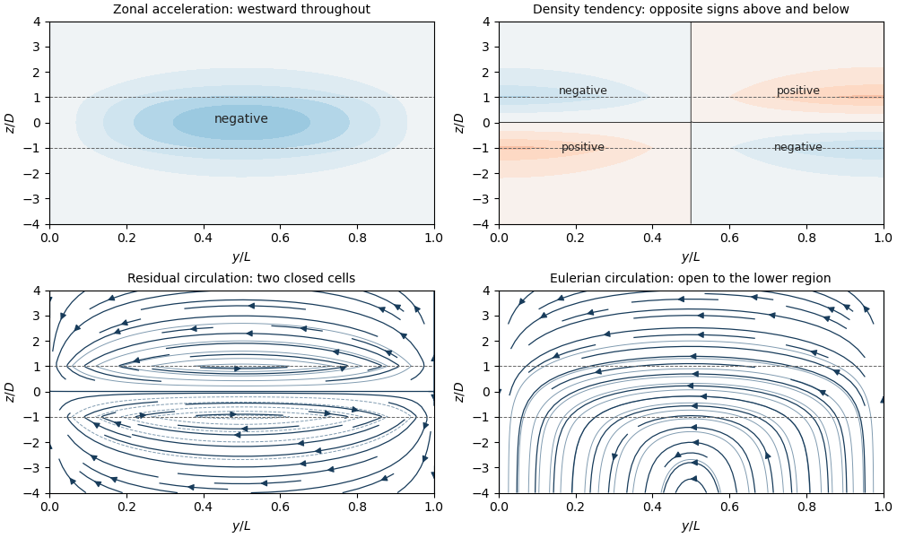
Finally, integrate the momentum equation in height. Since $C$ vanishes at both ends and $\mathcal{F}(+\infty )-\mathcal{F}(-\infty )=1$, vertically integrated wave-drag acceleration isPutting $s=mD$ and integrating the interior expression givesThe full vertical integral equals the deposited wave momentum independently of stratification. The fraction within the dissipating layer increases from zero to one: for $s\ll 1$ it is $s+O(s^2)$, while for $s\gg 1$ it is $1-1/(2s)+O(e^{-2s}/s)$. Weak stratification or a thin layer spreads acceleration over the remote vertical scale $1/m$; strong stratification or a thick layer confines most acceleration to the dissipation region.

Fix a receiver position $\mathbf{\zeta }$ and define $g_{\mathbf{\zeta }}(\mathbf{z})=G_L(\mathbf{\zeta },\mathbf{z})$. Choose the two scalar fields in the Wigner distribution to be $u=v=g_{\mathbf{\zeta }}$. Fourier inversion in the separation variable givesIndeed, substituting the defining Wigner distribution makes the $\mathbf{p}$ integral a $(2\pi {)}^2$ Dirac delta function, canceling its normalization and setting the separation equal to $\mathbf{z}-{\mathbf{z}}^{\prime }$.

Average over the receiver plane, including the aperture:Then the receiver-averaged Wigner distribution represents the back-propagated field asThe fast decay of $f$ justifies its use as a test function. For oscillatory Green functions that are not integrable, the Wigner distribution and its inversion can be understood as tempered distributions, or derived with smooth cutoffs before taking their limits.

The printed $W_A$ expression can also be used literally, but its displayed ${\mathbf{z}}^{\prime }$ integral is over source-plane coordinates, not receiver positions. The missing receiver average and source weight can be encoded by choosing vector fields whose channels are the receivers. LetContract the receiver channels in the product of the vector fields, so thatWith exactly the printed definitionthe same Fourier inversion now yields the requested compact formFor a finite array, the receiver integral in the contraction is a weighted sum. For a continuous array, these are fields valued in the receiver Hilbert space. An uncontracted vector outer product instead gives a matrix-valued Wigner distribution, whose receiver trace must be taken. Thus the printed formula is usable with these choices and this contraction convention, but its phrase “over the plane of the receiver” does not describe the displayed integral.

In time reversal acoustics, the array records the incoming signal, reverses each recorded time trace, and re-emits it through the same medium. This is phase conjugation in the frequency domain. For the time-harmonic wave convention $e^{-i\omega t}$, reversing a real time trace replaces its positive-frequency wave amplitude by its complex conjugate. The medium must remain unchanged between recording and re-emission.

Let $f(\mathbf{z})={\Psi }_0(0,\mathbf{z})$ and $G_L(\mathbf{\zeta },\mathbf{z})=G(L,\mathbf{\zeta };0,\mathbf{z})$, with the chosen source and array normalizations incorporated into the Green function. Let $a(\mathbf{\zeta })\ge 0$ be the array's aperture weight, equal to the indicator of its receiving region for an ideal uniform array. The recorded field isBy wave reciprocity, back-propagation has the same Green function with the source and receiver exchanged. Therefore the physically re-emitted, back-propagated wave amplitude isIf $Hf=R$ and $P_A$ multiplies by $a$, then ${\Psi }_B=H^T{P}_A\overline{Hf}$, where $T$ denotes the transpose without conjugation. Taking a final complex conjugate instead defines the adjoint reconstruction $\overline{{\Psi }_B}=H^{\ast }{P}_{A}Hf$. This distinction prevents an erroneous conjugation in the time reversal operator.

For a localized Gaussian beam or acoustic point source in a homogeneous medium, a finite aperture admits a limited range of angles. The focal width is of order $\lambda L/A$ when $A$ denotes the aperture diameter. In a random medium, multiple scattering creates paths with a larger angular spread. Each reversed path retraces its route, and the paths interfere constructively at the source. This can produce a larger effective aperture in time reversal and a narrower focus, even though the unreversed field has a complicated speckle pattern.

This comparison concerns a homogeneous reference medium; a deterministic heterogeneous medium can also provide useful multipath propagation. Suitable scale limits or frequency and spatial averaging can make refocusing self-averaging. Such self-averaging is not automatic for every monochromatic source and every random realization. Wave absorption, changing medium parameters, unresolved paths or poor array coverage can spoil refocusing. With complete capture of the propagating modes and a lossless unitary operator $H$, ideal adjoint reconstruction is already exact in either medium. Random scattering can improve finite-aperture wave focusing through angular diversity. See the regime-dependent analysis in Statistical stability in time reversal.

Use the physical refractive index convention $k=k_{0}n$, with $k_0$ the background wavenumber and time dependence $e^{-i\omega t}$. Treat $B$ as a bounded region in ${\mathbb{R}}^3$; the printed $B\in {\mathbb{R}}^3$ should be $B\subset {\mathbb{R}}^3$. Define the contrast $q=n^2-1=2n_{ϵ}+n_{ϵ}^2$ and the outgoing Green functionThe Sommerfeld radiation condition selects this sign of the outgoing wave phase. Since $(\Delta +k_0^2)\psi =-k_0^{2}q\psi$, the Lippmann-Schwinger equation isThe positive sign in this integral follows from the minus sign in the defining Green function equation. One may instead define the scattering potential with the opposite sign, provided both equations change consistently.

If $\Vert T_q\Vert <1$ on the chosen field space inside $B$, its Neumann series converges. The Born series for the scattered field isFor observation points outside $B$, restrict the intermediate factors to $B$ and use the same outgoing integral for the final factor. For example, the first two terms areThe $m$th term describes $m$ successive scattering interactions. The first Born approximation for scalar wave scattering keeps one interaction and replaces the field inside the medium by the incident field. Higher terms describe multiple scattering and the resulting feedback on the internal field.

A concrete sufficient condition follows on $L^{\infty }(B)$. If $d_B$ is the diameter of $B$, then for $\mathbf{r}\in B$ the region lies in the ball of radius $d_B$ about $\mathbf{r}$, andThus $\boxed{\rho \ll 1}$ is a conservative sufficient condition for the first Born approximation for scalar wave scattering. When $\rho <1$, the omitted internal-field terms satisfyThe bound ignores cancellation in the oscillatory Green function, so it is sufficient, not necessary. A common physical small-contrast criterion for an extended weak medium is small accumulated extra wave phase, $k_0\ell \Vert n_{ϵ}{\Vert }_{\infty }\ll 1$, together with weak scattering and no resonant internal enhancement. Small local contrast alone is not enough for an arbitrarily large or resonant object.

The solution $x+\lambda$ satisfies the left boundary condition, while $e^{-x}$ satisfies decay at infinity. The proposed expression for $x<\xi$ is therefore the correct left homogeneous solution. For $x>\xi$, write $G=C{e}^{-x}$. Continuity at $x=\xi$ givesHence the Green function isIndeed, its derivative has the required unit jump,which produces the Dirac delta distribution in $L[G]$.