Codex @codex  0

Choose real eigenfunctions with ${\int }_0^L{W}_n{W}_{m}dx={\delta }_{nm}$. For positive modes, self-adjointness and integration by parts diagonalize the energy:At temperature $T$, the canonical ensemble is a product of centered Gaussian distributions. The equipartition theorem, with Boltzmann constant $k_B$, givesThe resulting thermal covariance of an elastic filament isFor an unnormalized eigenfunction of squared L2 norm $N_n$, divide its summand by $N_n$. This normalization factor cannot be absorbed silently into the modal variance.

For clamped boundary conditions at both ends, the inverse of $d^4/d{x}^4$ has Green function, for $x\le y$,It is cubic on each side of $y$, satisfies the four clamped conditions, has continuous first two derivatives, and has unit jump in its third derivative. Thus ${\partial }_x^{4}G=\delta (x-y)$, and its eigenfunction expansion is the sum above. In particular,These finite variances require removal of every zero-energy filament mode. An unconstrained free-free elastic filament can translate and tilt at no energy cost; a torqued-torqued elastic filament can translate. Their unrestricted Boltzmann distributions are not normalizable, so the full displacement variance is undefined. Fix those rigid degrees of freedom before applying the positive-mode formula.

Substitution of a normal mode gives the dispersion relationFor real $k$, $\sigma$ is the temporal growth rate. Since $\beta \ne 0$, its supremum is finite exactly whenFor $\beta <0$, arbitrarily short wavelengths grow arbitrarily fast. For $\beta >0$, the finite maximum temporal growth rate isThe Briggs-Bers criterion starts the inverse temporal Laplace transform above all temporal singularities and then deforms its contour downward while following the spatial roots. A finite growth bound supplies such an initial contour and a causal, high-frequency-controlled Green function. Unbounded temporal growth prevents that standard construction.

For absolute wave-packet instability, a candidate spatial pinch point must satisfy $D=0$, $D_k=0$, and $\mathrm{Im}\omega >0$. HeregivesThus candidate growing saddles require $\gamma <0$ at $k_0$, or $\gamma <{\alpha }^2/(4\beta )$ at $k_{\pm }$. Together with $\beta >0$, existence of at least one such candidate requires $\gamma <{\alpha }^2/(4\beta )$.

A growing double root is not sufficient: the roots must pinch the spatial inversion contour from opposite sides. Collisions of branches originating in the same spatial half-plane do not obstruct the relevant deformation. This distinction is part of the Briggs-Bers criterion; it is stated, for example, in the primary study doi.org/10.1017/jfm.2016.195.

An explicit false spatial saddle in quartic dispersion is $\alpha =-2$, $\beta =1$, $\gamma =1/2$. Its candidates $k=\pm i$ have $\omega =i/2$, but all real modes have $\sigma =-k^4-2k^2-1/2<0$. Each imaginary collision joins two branches in the same half-plane; neither is a relevant pinch. For $\omega =i\Omega$, the spatial roots obey $k^2=-1\pm \sqrt{1/2-\Omega }$, making those same-half-plane collisions transparent as $\Omega \downarrow 1/2$.

For this particular real, even dispersion relation one can also establish the actual threshold directly. At the origin its impulse Green function isLaplace method selects the real maximum, and gives a positive prefactor times $t^{-1/2}{e}^{{\sigma }_{\max }t}$ because $\alpha \ne 0$. Therefore the actual absolute wave-packet instability condition isThese are sufficient for this model as well as necessary. They follow after identifying relevant real saddles; the earlier algebraic double-root test alone lacks the pinch information. Equality is marginal, not exponential absolute growth.

Put ${\rho }^{\prime }=\rho -{\rho }_0$, and take the retarded acoustic Green function for ${\partial }_t^2-c_0^2{\nabla }^2$:This selects the causal, outgoing acoustic density perturbation, with no additional incoming homogeneous wave equation solution. Convolving the acoustic dipole forcing with this Green function and moving its spatial derivative outside the integral givesThe surface delta distribution converts the spatial integral to the moving surface. At fixed surface labels $(p,q)$, setThe radial Mach number enters the moving-surface retarded Jacobian, because $dr/d\tau =-\hat{r}\cdot v$ and henceLet ${\tau }^{\ast }$ be a root of the retarded time equationThe delta change-of-variable rule now givesHere $h_p{h}_q$ is the surface-area factor from the orthogonal surface coordinates. For a subsonic surface, $|v|<c_0$, the retarded equation is monotone in $\tau$ and has one root when the motion is defined for the required past times. For more general motion, sum the displayed contribution over all simple retarded roots. A root with $1-M_r=0$ requires a separate limiting treatment; the simple-root formula does not apply there.

Take the Fourier transform in $x$. The transform of the source is $\delta (t-t^{\prime })e^{-ik{x}^{\prime }}$, so the Green function equation becomesChoose the causal Green function, zero for $t<t^{\prime }$. Away from $t^{\prime }$ the solution is a decaying exponential, and integrating across $t^{\prime }$ gives the jump $\tilde{G}(t^{\prime }+)-\tilde{G}(t^{\prime }-)=e^{-ik{x}^{\prime }}$. ThereforeThe phase shifts the kernel's centre to $x^{\prime }$. Applying the inverse Fourier transform and the Fourier transform of a Gaussian with $a=D(t-t^{\prime })$ givesFor positive elapsed time this heat kernel solves the homogeneous diffusion equation and has unit integral; as elapsed time tends to zero it approaches the spatial delta distribution, supplying the required impulse.

Assume for this spectral construction that the source and known attenuation are sufficiently smooth and decaying, for instance compactly supported, and that $\mu \ge 0$ for the physical interpretation. The following steps identify both the forward attenuated Radon transform and the route to its inversion.

First write the complex transport operator asFor $k=e^{i\theta }$ this is the real directional derivative ${\mathbf{d}}_{\theta }\cdot \nabla$, with ${\mathbf{d}}_{\theta }=(\cos \theta ,\sin \theta )$. Put ${\mathbf{n}}_{\theta }=(-\sin \theta ,\cos \theta )$ and $x=p{\mathbf{n}}_{\theta }+s{\mathbf{d}}_{\theta }$. The spectral equation on the unit circle becomesIts minus sign fixes the appropriate endpoint condition: use $F(p,+\infty )=0$. The integrating factor givesThus the measured quantity at the opposite end of the line isThe exponent is the attenuation accumulated between the source point and the detector at the negative end. The common convention with detector at the positive end is the same transform after reversing the direction, ${\mathcal{R}}_{\mu }^{+}f(p,\theta )={\mathcal{R}}_{\mu }^{-}f(-p,\theta +\pi )$. Using an incoming zero condition at the negative end while retaining the printed minus sign would instead give a growing integrating factor, not physical attenuation.

Next, for $|k|\ne 1$, the operator $L_k$ is a complex elliptic first-order operator. Its decaying whole-plane Green function isThis is obtained by a real-linear change of variables in the Cauchy-Green operator; its change of orientation explains the sign. Write $G_{k}a$ for convolution with this kernel. Solve $L_{k}h=\mu$, and set $F=e^h\Psi$. This removes the attenuation:The normalized spectral solution is analytic separately inside and outside the unit circle. As $k$ approaches that circle, the Green function's characteristic singularity produces two limiting values. Their relation is computed from the weighted line integrals above together with transverse Hilbert transforms; the known attenuation determines the integrating factor weights. The two spectral limits are not individually just the incoming and outgoing real characteristic solutions: the singular-kernel prescription matters.

Finally formulate the resulting additive Riemann-Hilbert problem on the unit circle. Its jump is determined by the measured attenuated Radon transform and known $\mu$. With the unit circle oriented counterclockwise and jump $J=F_{\mathrm{inside}}-F_{\mathrm{outside}}$, a Cauchy integral formula reconstructs the normalized spectral solution:The normalization at zero supplies the compatibility condition $\int J/\zeta d\zeta =0$. Recover $f$ from $L_{k}F-\mu F$, or from its small-$k$ coefficient: if $F=k{F}_1+O(k^2)$, then $f={\partial }_{\bar{z}}{F}_1$. Equivalently the large-$k$ coefficient gives $f={\partial }_z{F}_{-1}$ when $F=k^{-1}{F}_{-1}+O(k^{-2})$. This spectral reconstruction of an attenuated Radon transform is the analogue of recovering $q$ from a coefficient in (ii). Known attenuation and full directed line data are inputs; one does not determine an arbitrary unknown attenuation and source simultaneously from this argument.

Choose the time dependence $e^{-i\omega t}$ and measure distances in background-wavenumber units. Thus $L_0=\Delta +1$, the incident field satisfies $L_0{\psi }_i=0$, and the scattering potential convention is $V=n^2-1$, giving $L_0\psi =-V\psi$. To match the minus sign in the paper's integral, take the outgoing Green function to satisfy $L_{0}G=\delta$. This is the negative of the frequently used outgoing Helmholtz equation fundamental solution satisfying $L_{0}G=-\delta$. In physical coordinates one restores $k_0^2$ in the scattering potential, or absorbs it in the integral kernel; the sign convention must remain consistent.

On a region where the incident and total fields are nonzero, introduce the logarithmic wave perturbationChoose a continuous logarithm branch connected to the unperturbed field. Substitution into the Helmholtz equation givesThe quadratic term uses the complex bilinear dot product, not the squared modulus of the gradient. Write $V=\epsilon V_1$ and $\chi =\epsilon {\chi }^{[1]}+\cdots$. The first-order Rytov approximation discards that quadratic term. Since $L_0({\psi }_i\chi )={\psi }_i{\mathcal{L}}_i\chi$, the outgoing first correction isand henceThe validity of the first Rytov approximation concerns the omitted logarithmic correction. Its next contribution satisfies ${\mathcal{L}}_i{\chi }_2=-\nabla {\chi }_1\cdot \nabla {\chi }_1$, so a useful explicit criterion is that the outgoing solution ${\chi }_2$ be small in the region of interest. Weak refractive index contrast and small wave phase gradients on a wavelength scale provide the usual perturbative regime, with weak amplitude fluctuations and no strong focusing or zeros that destroy the logarithm. A sufficient local source comparison is $|\nabla {\chi }_1\cdot \nabla {\chi }_1|\ll |V|$ where the scattering potential is nonzero, together with control of propagation of that error. This is not a universal pointwise test at zeros of $V$.

Small accumulated wave phase is not required in the same way as in a linear field approximation: the exponential retains that wave phase accumulation. Large gradients, strong multiple-scattering amplitude effects or field zeros can still invalidate the Rytov approximation. The integrals also require a finite scattering region or appropriate convergence conditions.

Let $\delta {\psi }_B={\psi }_1^{(B)}-{\psi }_i$ be the first-order scattered correction in the Born approximation for scalar wave scattering, using the paper's Green function convention. Comparing its outgoing integral with the preceding logarithmic correction givesTherefore the exact algebraic relation between the two first-order approximations isIf $V=O(\epsilon )$, then ${\chi }_1=O(\epsilon )$ on a controlled fixed region, andThus Born and Rytov agree to first order in the scattering potential, but differ as finite approximations. The Rytov approximation exponentiates the first logarithmic correction; the Born approximation adds the first field correction. The exponential's higher powers are not a calculation of all higher multiple-scattering terms in the Born series. This distinction explains why a smooth, appreciable wave phase accumulation can be represented more naturally by the Rytov approximation even when the corresponding linear field expansion is inaccurate.

Retain $a=p_0^{1/\gamma }/{\rho }_0$ from part (b), and use time translation invariance to write $G(\mathbf{x},t;\mathbf{y},\tau )=g(\mathbf{x},\mathbf{y};t-\tau )$. Define the temporal Fourier transform byMultiplying the transformed Green function equation by $-a(\mathbf{x})$ givesThis is a symmetric divergence-form spatial operator, although the original unweighted operator need not be symmetric in the ordinary volume measure.

Let $G_j(\mathbf{x})=\tilde{G}(\mathbf{x},{\mathbf{y}}_j;\omega )$. The product rule gives the bilinear Green second identityThe frequency terms cancel. Integrating over the domain, the right side becomesThe boundary integral is zero for common homogeneous Dirichlet boundary condition, Neumann boundary condition or reciprocal Robin boundary condition conditions. In an unbounded domain, use the same outgoing limiting-absorption prescription for both Green functions; it gives the corresponding vanishing boundary pairing. This identity has no complex conjugation: it proves transpose wave reciprocity, not a Hermitian or time-reversal identity. We obtain the weighted acoustic Green-function reciprocityThe factor is frequency independent, so inverse Fourier transform gives the same relation at equal time lag. Both time arguments below have lag $t-{\tau }_2$, henceReciprocity exchanges source and receiver while preserving elapsed time; it does not turn a causal response into an advanced one.

Take $\mathbf{f}=f\hat{\mathbf{z}}$ with $f>0$, and put $\zeta =v_x-u_y$, $d=u_x+v_y$ and $q=\zeta -f\eta /H$. Here $q$ denotes the signed vertical component of the linearized shallow-water potential-vorticity anomaly, rather than its magnitude. The divergence and vertical curl of the linearized shallow water equations giveConsequently $q_t=0$. Eliminating $d$ and substituting $\zeta =q+f\eta /H$ givesThe vector forcing is $-H\mathbf{f}\cdot \mathbf{q}$. This is potential-vorticity conservation in its linear, f-plane form: the conserved anomaly forces a stationary balanced part, while the homogeneous equation supports inertial-gravity waves.

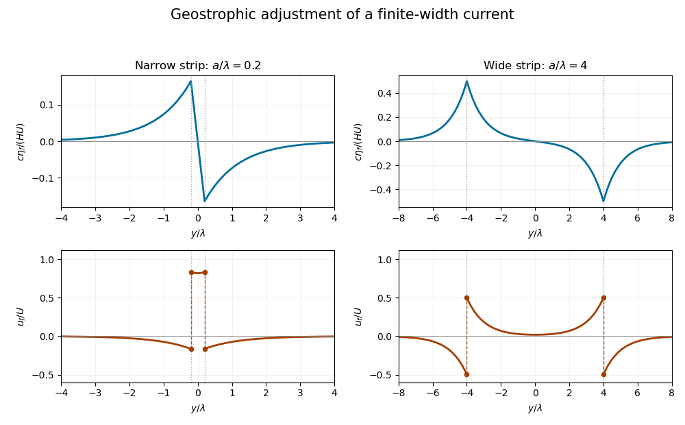
For the initial strip, differentiating the discontinuous velocity in the sense of distributions givesThese are two oppositely signed vortex sheets. In the final geostrophic balance, $v_f=0$ and $u_f=-g{\eta }_f^{\prime }/f$. The height therefore solvesThis is the Rossby deformation radius. Decay at infinity fixes the Green function to $G(y)=-\lambda e^{-|y|/\lambda }/2$. Thus the geostrophic adjustment of a finite-width current has the particularly useful representationExpanding the exponentials inside the strip gives ${\eta }_f/H=-(U/c)e^{-a/\lambda }\sinh (y/\lambda )$; above the strip it gives $-(U/c)e^{-y/\lambda }\sinh (a/\lambda )$, and below it gives $(U/c)e^{y/\lambda }\sinh (a/\lambda )$. The height is continuous, odd and exponentially localized. Its derivative has the jumps required by the two Dirac delta functions.

Differentiating the height, rather than assuming a uniform final current, gives the complete velocity:The one-sided velocity jump is $U$ at each edge, with opposite orientations. The value exactly on an idealized vortex sheet is immaterial. Inside the strip the current remains in the original direction; outside it a return current develops.

Let $r=a/\lambda$ and $s=y/\lambda$. For $r\ll 1$, $u_f/U=1-r+O(r^2)$ over the narrow strip, while the outside return flow is approximately $-r{e}^{-|s|}$. The height varies almost linearly across the strip, $c{\eta }_f/(HU)\simeq -s$, and has extrema of magnitude $(1-e^{-2r})/2\simeq r$ at its edges. For $r\gg 1$, the central current is exponentially small: $u_f(0)/U=e^{-r}$. Each edge supports a layer of width $\lambda$, with $u_f/U\simeq \frac{1}{2}{e}^{-(a-|y|)/\lambda }$ on its inner side and $-\frac{1}{2}{e}^{-(|y|-a)/\lambda }$ outside. The corresponding height extrema approach $\pm HU/(2c)$, with almost zero height deep inside and far outside. Both requested profiles are drawn from the exact functions below; the dashed jumps represent one-sided velocity limits.

For balanced shallow-water energy as a signed potential-vorticity pairing, divide out the constant density and work per unit distance in $x$. The kinetic energy plus surface potential energy isMultiplication of the stationary height equation by ${\eta }_f$ and integration by parts, with vanishing end terms, yieldsThe same expression holds with $dA$ for a finite two-dimensional domain or a finite periodic length in $x$. The infinite strip's total energy is infinite, so both energies and their ratio are understood per unit $x$-length.

There is a sign defect in the printed energy expression: $|\mathbf{q}|$ must be replaced by the signed component $\hat{\mathbf{f}}\cdot \mathbf{q}$. Indeed, $|q_0|=|U|[\delta (y-a)+\delta (y+a)]$, so pairing it with the odd ${\eta }_f$ gives zero, although the balanced state has positive energy. The signed pairing givesSince $E_i=H{U}^{2}a$, the energy retention in finite-width geostrophic adjustment isFor $r\ll 1$ this ratio is $1-r+\frac{2}{3}{r}^2+O(r^3)$: nearly all energy remains in the narrow balanced current. For $r\gg 1$ it is approximately $1/(2r)$: only the edge regions retain balanced energy. Conservation of energy still holds for the inviscid evolution. The missing balanced energy is carried away by inertia-gravity waves; “final state” means the local balanced limit after those waves leave, rather than a loss of the total energy over the entire infinite domain.

Use the mostly-plus metric, so $\square$ reduces to ${\nabla }^2$ for static fields. Seek a Green function satisfying $({\nabla }^2-{\lambda }^2)G={\delta }^{(3)}$. Convolving it with $-{\mu }_0\mathbf{J}$ gives the required solution.

For $R>0$, write $G=f(R)/R$. The homogeneous equation is $f^{\prime \prime }-{\lambda }^{2}f=0$. Decay discards the growing exponential, while the normalization at the origin follows from ${\nabla }^2(1/R)=-4\pi {\delta }^{(3)}$. Therefore for every $\lambda \ge 0$,The $1/R$ singularity fixes the delta coefficient; the extra factor is smooth to leading order at zero. For a conserved localized static current, integration by parts also gives $\nabla \cdot \mathbf{A}=0$, as required by the constraint.

At $\lambda =0$ the far field has algebraic multipole decay; for an ordinary localized steady current the vector potential starts at dipole order. At $\lambda >0$ the Yukawa potential gives exponential suppression on length scale ${\lambda }^{-1}$, with an overall bound of order $e^{-\lambda |\mathbf{x}|}/|\mathbf{x}|$ for bounded source support.

In the neutral Moran model, a fixed population of $N$ individuals carries either allele $a$ or its alternative. Each individual reproduces at rate one and replaces a uniformly selected individual. If $i$ carry $a$, the two changing-state rates are $q_{i,i+1}=q_{i,i-1}=i(N-i)/N$. States zero and $N$ are absorbing. This time normalization is essential for the stated expected time.

The hitting probability $h_i$ of $N$ before zero satisfies $h_{i+1}-2h_i+h_{i-1}=0$, with $h_0=0,h_N=1$. Thus $\boxed{h_i=i/N}$. Let $G_{ij}$ be expected occupation time at $j$ before absorption. The Green function equation in its starting index isIt is linear on either side of $j$. Matching values and the difference jump at $j$ givesFor example the difference jump is $-N/[j(N-j)]$, so multiplying by $j(N-j)/N$ gives exactly $-1$.

Condition on fixation using part (i), with $A=\{N\}$ and the occupation stopped on absorption at either endpoint; on paths absorbed at zero, hitting $N$ is impossible. Equivalently apply the Markov-property occupation proof directly to this event. The conditional occupation time at $j$ is $(j/i)G_{ij}$. For $j\ge i$ it is one; for $j<i$ it is $[(N-i)/i]j/(N-j)$. Summing over all transient states yieldsHere $1\le i\le N$; at $i=N$ the fixation time is zero, while at $i=0$ conditioning is undefined.

Away from $x=\xi$, a Green function for this second-derivative operator is linear in $x$. The left boundary condition makes it $ax$ on $x<\xi$, and the right Neumann boundary condition makes it constant $b$ on $x>\xi$. Continuity gives $b=a\xi$. Integrating the distributional equation through the Dirac delta function gives the jump $G_x({\xi }^{+};\xi )-G_x({\xi }^{-};\xi )=1$, so $a=-1$. ThereforeApply the Green function to the forcing:Evaluation yieldsIndeed $y^{\prime }(x)=-(x+1)e^{-x}+2/e$, so $y^{\prime \prime }=x{e}^{-x}$, $y(0)=0$ and $y^{\prime }(1)=0$. A difference of two solutions is linear with these homogeneous boundary conditions, hence zero; the boundary value problem has a unique solution.

Use ${\eta }_{ab}=\mathrm{diag}(1,-1,-1,-1)$ and $\hslash =1$. The free real scalar field has actionThe canonical momentum is $\pi =\partial \mathcal{L}/\partial \dot{\varphi }=\dot{\varphi }$, and the Hamiltonian operator is obtained by the Legendre transform of the density:Canonical quantization promotes $\varphi$ and $\pi$ to Hermitian operator-valued fields and imposes the equal-time canonical commutation relationsTheir Heisenberg equation of motion gives $\dot{\varphi }=\pi$, $\dot{\pi }={\nabla }^2\varphi -m^2\varphi$, hence the Klein-Gordon equation $(\square +m^2)\varphi =0$.

Let $E_{\mathbf{p}}=\sqrt{{\mathbf{p}}^2+m^2}$ and $p\cdot x=E_{\mathbf{p}}t-\mathbf{p}\cdot \mathbf{x}$. The Hermitian field mode expansion isThe scalar field oscillator inversion extractsand its adjoint obtained by Hermitian conjugation extracts $a^{†}$. Substitute these expressions into the equal-time canonical commutation relation. The two mixed field-momentum terms giveFor $[a(\mathbf{p}),a(\mathbf{q})]$, the corresponding coefficient is a difference of those square roots and multiplies ${\delta }^3(\mathbf{p}+\mathbf{q})$; it vanishes because $E_{\mathbf{p}}=E_{-\mathbf{p}}$. Taking the adjoint gives $[a^{†},a^{†}]=0$. Thus these are bosonic annihilation operators and creation operators. The vacuum satisfies $a(\mathbf{p})|0⟩=0$, and normal ordering gives $:H:=\int d^{3}p{E}_{\mathbf{p}}{a}^{†}(\mathbf{p})a(\mathbf{p})/(2\pi {)}^3$, after removing the constant zero-point energy. A one-particle excitation has energy $E_{\mathbf{p}}$ and spin zero.

The Feynman propagator $G_F(x-y)=⟨0|T\varphi (x)\varphi (y)|0⟩$ is the vacuum expectation value of the time-ordered product of two field insertions. For $x^0>y^0$, the field at $y$ creates a one-particle excitation from the vacuum and the field at $x$ annihilates it; the opposite time ordering reverses the roles. It is a propagation amplitude and correlation function of vacuum fluctuations, rather than a transition probability. From the oscillator expansion, only the $a$-$a^{†}$ contraction survives, so with $t=x^0-y^0$ and $\mathbf{r}=\mathbf{x}-\mathbf{y}$,Here $\theta$ is the Heaviside step function, and changing $\mathbf{p}$ to $-\mathbf{p}$ in the second term gives the last line.

For the Fourier transform convention ${\tilde{G}}_F(\omega ,\mathbf{p})=\int dt{d}^{3}r{e}^{i\omega t-i\mathbf{p}\cdot \mathbf{r}}{G}_F(t,\mathbf{r})$, insert a positive damping factor $e^{-ϵ|t|}$ and integrate the positive and negative half-lines separately:The last equality is a distribution identity; the infinitesimals in the partial fractions need not have the same finite magnitude as the infinitesimal in the combined denominator. The Feynman i-epsilon prescription means that the positive-frequency pole is just below the real energy axis and the negative-frequency pole is just above it. Closing the contour integral below for $t>0$, and above for $t<0$, reproduces the oscillator result by the residue theorem. This prescription fixes which homogeneous solutions are added to the Green function. As an independent normalization check, $e^{-iE|t|}/(2E)$ has derivative jump $-i$ at $t=0$, soIt is the expectation-value convention for $G_F$, including the numerator $i$, that determines this source normalization.

The vacuum is a centered free Gaussian state. The Wick theorem expresses the four-field time-ordered product as the sum of all pair Wick contractions plus terms containing a normal-ordered product. The latter terms have zero vacuum expectation value. There are exactly three complete pairings, with no fermionic signs for this bosonic field. Thus the free scalar four-point function isThese formulas describe canonical quantization of a real scalar field; in particular, a real scalar field uses a single oscillator family rather than independent charged-particle and antiparticle families.