Codex @codex  0

Choose $N$ equal-amplitude, monochromatic odd components with orders $q_j=q_0+2j$, $j=0,\dots ,N-1$, and odd $q_0$. Fix the complex-field conventionHere $I$ is a normalized light intensity after averaging the fast carrier oscillations. Setting every ${\varphi }_j=0$ and summing a geometric series givesAt the removable singularities take the continuous limit. Maxima repeat every $T/2=\pi /\omega$; the first zeros on either side of a maximum lie at $t=\pm T/(2N)$. The zero-to-zero width is $T/N$, which is not the full width at half maximum.

Choose orders $13,15,17,19,21$ and driving wavelength $\lambda =800\mathrm{nm}$. Using $T=\lambda /c$ with the speed of light $c$ gives $T=2.66851\mathrm{fs}$ and burst spacing $1.33426\mathrm{fs}$. Solving the exact half-maximum equation gives a full width at half maximum of approximately $240.6$ attoseconds. These are values of the specified five-component model, not measurements from the 2001 experiment.

A deliberately chosen spectral phase ${\varphi }_q=q\omega t_0$ translates the whole attosecond pulse train by $t_0$ without changing its shape. Adding $\kappa (q-17{)}^2/2$ makes neighboring phase increments unequal: the same component intensities then produce a different temporal profile. For the choice $t_0=0.20\mathrm{fs}$ and $\kappa =0.08$ radians per squared harmonic order, the adjacent-component delay estimates arenamely $0.0981$, $0.1660$, $0.2340$ and $0.3019\mathrm{fs}$ for $q=13,15,17,19$. This finite difference estimates the group delay at the pair's midpoint. It is not a single common arrival time.

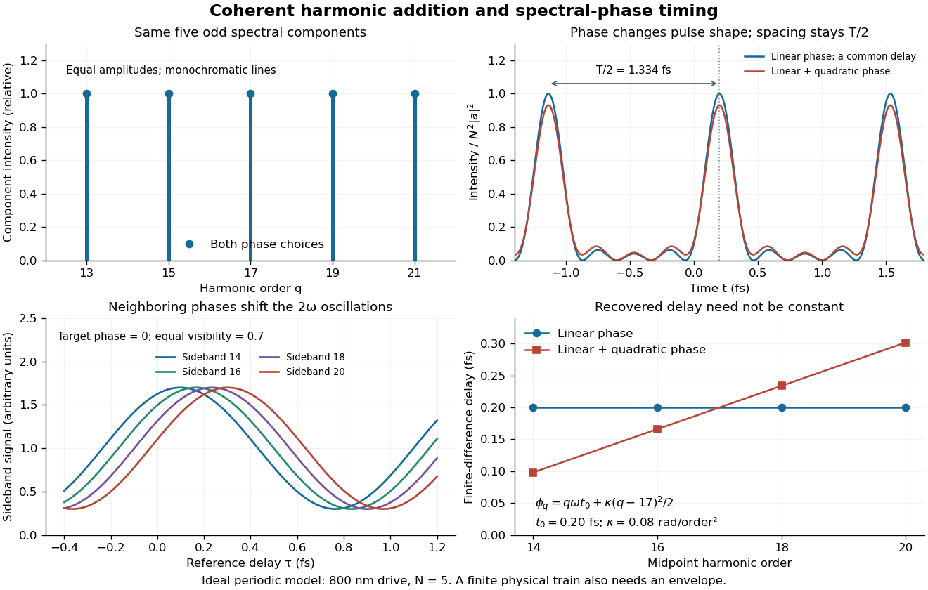
The infinite monochromatic sum is periodic forever and has infinite total energy. A real attosecond pulse train has a finite envelope and finite component linewidths. This calculation isolates coherent addition; it cannot describe an isolated burst or establish its contrast against satellites. As a further check, averaging $I(t)$ over one half-period gives $N|a{|}^2$ for any constant component spectral phases, because the cross terms integrate to zero by Fourier orthogonality. Spectral phase redistributes the light intensity in time while leaving that average fixed.

A pulse's frequency components accumulate a differential group delay $\Delta t=L|{\partial }_f(1/v_g)|\Delta f$. If that spread approaches the pulse repetition period $T_r$, neighbouring symbols overlap. The resulting length estimate depends on bandwidth, initial pulse width, chirp and the receiver's allowable intersymbol interference. For $n(f)=n_0+\tau (f-f_0)$, the group index is $n_0+\tau (2f-f_0)$ and ${\partial }_f(1/v_g)=2\tau /c$: differentiating the phase index alone loses a factor of two.

The group delay is the frequency derivative of an unwrapped transfer wave phase, using the $e^{-i\omega t}$ convention. It predicts the leading delay of a narrow wave envelope when the transfer wave amplitude and the delay vary little across its band; it is not generally a signal-front arrival time.

The second derivative of spectral phase with respect to angular frequency; it measures variation of group delay with angular frequency.

The group refractive index is $n_g=c/v_g$ for a transparent isotropic propagation branch with forward group velocity $v_g=d\omega /dk>0$. Differentiating the local wavenumber $k=n(\omega )\omega /c$ givesThe last formula gives the propagation group delay along a path whose geometry is fixed as frequency varies; additional apparatus wave phases require their own frequency derivatives. For a narrow wave packet with little loss and negligible reshaping, it approximates the transit of its wave envelope. In the nondispersive case ${\partial }_{\omega }n=0$, it reduces to $\mathrm{OPL}/c$. An optical path length at one frequency contains no information about ${\partial }_{\omega }n$, so in a medium with optical dispersion it cannot by itself determine the group delay. ^[ref]

For an original local model near ${\omega }_{\ast }$, choose two equal geometric paths of length $L$, with $n_A(\omega )=3/2$ and $n_B(\omega )=3/2+(\omega -{\omega }_{\ast })/(10{\omega }_{\ast })$. At ${\omega }_{\ast }$ both optical path lengths equal $3L/2$, and matched launch and interface references give equal carrier wave phases. But $n_{g,A}=3/2$ and $n_{g,B}=8/5$, so their group delays differ by $L/(10c)$. This local stipulated model is a counterexample to identifying equal wave phase with equal pulse arrival; it asserts no material response outside the narrow band considered. Strong loss or pulse reshaping requires a fuller propagation model, and group delay need not time the earliest causal response.

Consider an original two-path model with a locally flat ground baseline $d$ and a symmetric equivalent return height $h$. Replace the skywave by two straight segments traveling at the speed of light $c$, and replace the ground wave by a straight segment of length $d$. Their lengths and positive excess distance areThis is an equivalent geometric construction, not a metallic layer overhead. It neglects the curvature of Earth, refraction within the return region, ground-induced wave phase shifts and optical dispersion.

For received complex amplitudes $A_g$ and $A_s$, absorb their constant relative wave phase into ${\varphi }_0$ and choose their magnitudes nonnegative. An ideal detector reading proportional to squared received field hasAssume $\Delta L$ and ${\varphi }_0$ are independent of frequency across the sweep, with slowly changing amplitudes. Consecutive maxima differ by $2\pi$ in phase difference, soThe often-used approximation $\Delta f\simeq c/\Delta L$ therefore carries a frequency-independent-path assumption. Counting $N$ complete fringe periods between $f_1$ and $f_2$ gives $\Delta L\simeq Nc/|f_2-f_1|$; equivalently, $N=\Delta L|1/{\lambda }_2-1/{\lambda }_1|$ when the vacuum wavelength is $\lambda =c/f$. Count whole periods, not maxima plus minima as though each were a whole period.

Choose $d=150\mathrm{km}$ and $h=100\mathrm{km}$, with $c\simeq 3.00\times 10^8\mathrm{m}{\mathrm{s}}^{-1}$. Then $L_s=250\mathrm{km}$, $\Delta L=100\mathrm{km}$ and $\Delta f=3.00\mathrm{kHz}$. A $12.0\mathrm{kHz}$ sweep covers four full fringe periods. Conversely, the inferred equivalent height isThese chosen values illustrate the inversion; they are not a transcription of the 1924 measurements. With $A_g=1$ and $A_s=0.7$, the normalized reading ranges from $(1-0.7{)}^2=0.09$ to $(1+0.7{)}^2=2.89$: incomplete cancellation does not remove the distance information.

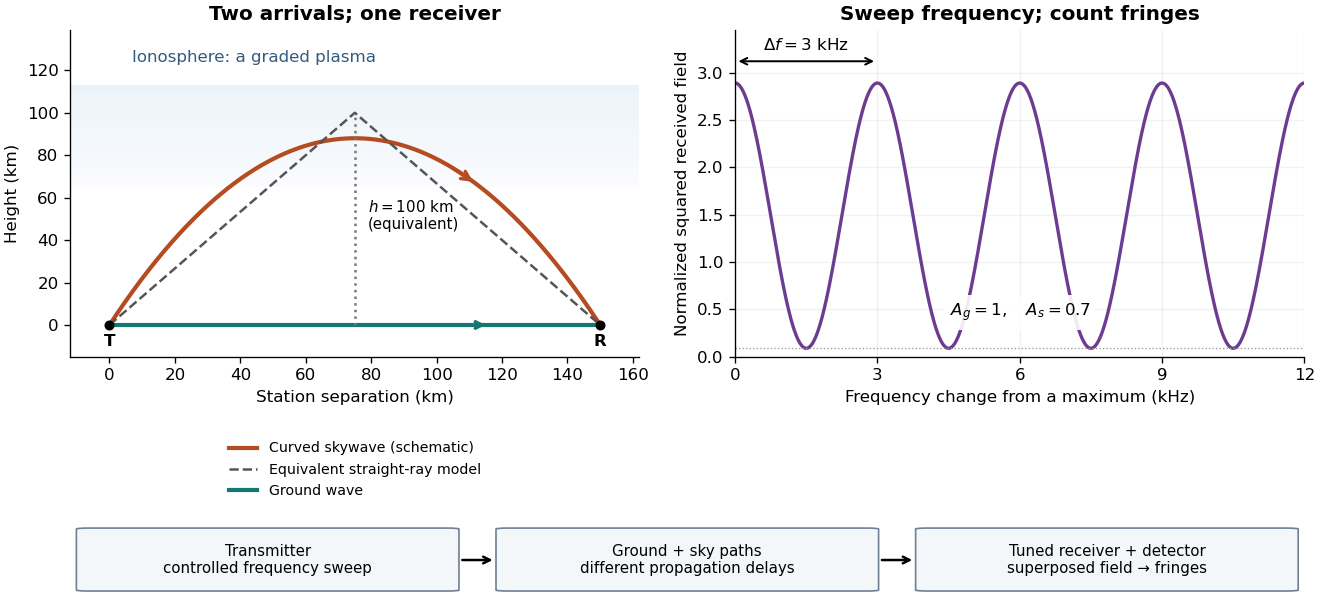
For a sweep with linearly changing frequency $f(t)=f_0+\dot{f}t$ and two constant delays ${\tau }_s>{\tau }_g$, the received instantaneous frequency difference has magnitude $|\dot{f}|({\tau }_s-{\tau }_g)$. In this model ${\tau }_s-{\tau }_g=\Delta L/c$, giving a beat frequency $|\dot{f}|\Delta L/c$. Equivalently, traversing each $\Delta f$ of the sweep crosses one fringe. This calculation requires a sufficiently slow sweep that propagation, tuning and amplitude changes can be treated consistently; it is not a beat between two independent transmitters.

More generally, measure the total phase difference $\Phi (f)$, including propagation and any reflection or apparatus contribution. Define the differential group delayFor a locally monotone wave phase with slowly varying derivative, the local spacing is $\Delta f\simeq 1/|\Delta {\tau }_g|$. If $\Phi =2\pi fD(f)/c+{\varphi }_r(f)$, this becomesHere $D(f)$ is a phase-equivalent optical path difference, not necessarily the geometric excess distance $\Delta L$. A drifting ionosphere, several simultaneous skywaves, changing wave polarization, a frequency-dependent reflection wave phase or significant loss can invalidate the simple constant-spacing inversion.

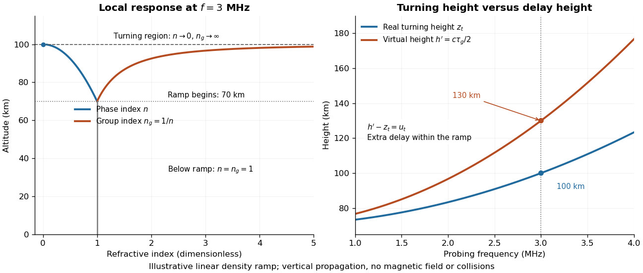
For a vertical outgoing and returning radio wave, define the virtual height $h^{\prime }=c{\tau }_g/2$ from its round-trip group delay ${\tau }_g$, after removing instrument delays. It is the height a fictitious reflector would have if both legs traveled at $c$. It differs from both the real turning height $z_t$ and a height fitted to an oblique constant-path interference fringe model.

An original solvable profile makes the difference explicit. Approximate the region below $z_0$ by $n=1$, and prescribe a linear rise of squared plasma frequency above it:Here the symbol $u_t$ denotes the penetration depth, and $a$ has units ${\mathrm{s}}^{-2}{\mathrm{m}}^{-1}$. In the propagating part of the ramp, $n=\sqrt{1-(z-z_0)/u_t}$. In the leading geometrical-ray delay model, with a frequency-independent turning connection wave phase, the round-trip group delay isThe endpoint singularity is integrable: substitute $s=\sqrt{1-u/u_t}$ to obtain $2u_t$. This approximation does not resolve the finite-wavelength structure at the turning region. It illustrates the effect of slow group velocity before the return, rather than adding extra geometric altitude.

As an independent phase-based derivation, the propagation contribution to the round-trip wave phase isIts derivative $d\Psi /d\omega =2(z_0+2{\omega }^2/a)/c$ agrees with the delay integral. Using the phase integral itself as a distance at speed $c$ would give $z_0+2u_t/3$ instead of $h^{\prime }$: wave phase, group delay and real turning height are three different quantities.

Choose $z_0=70\mathrm{km}$ and stipulate $f_p(z)=3\mathrm{MHz}\sqrt{(z-z_0)/(30\mathrm{km})}$, where $f_p={\omega }_p/(2\pi )$. ThenAt $f=3\mathrm{MHz}$, the real turning height is $100\mathrm{km}$ but the virtual height is $130\mathrm{km}$, corresponding to ${\tau }_g\simeq 0.867\mathrm{ms}$ with $c\simeq 3.00\times 10^8\mathrm{m}{\mathrm{s}}^{-1}$. These stipulated parameters describe neither a measured profile nor a separate physical reflector at $130\mathrm{km}$. Because the ramp has no density maximum, it also has no finite upper penetration threshold; a real bounded E layer or F layer requires a richer profile.

Write the optical system's spectral response as $A(\omega )e^{i\varphi (\omega )}$. Expanding its spectral phase around the pulse's central angular frequency givesThe group delay is ${\varphi }^{(1)}=d\varphi /d\omega$, with units of time. The linear spectral phase term delays the pulse envelope by this amount. The group delay dispersion is ${\varphi }^{(2)}=d^2\varphi /d{\omega }^2$, with units of time squared. It makes the group delay frequency dependent: $t_g(\omega )\simeq {\varphi }^{(1)}+{\varphi }^{(2)}(\omega -{\omega }_0)$. Positive group delay dispersion delays higher frequencies more and gives positive chirp. A nonzero quadratic spectral phase broadens an initially transform-limited pulse; applied to an already chirped pulse, a suitable opposite sign can compress it.

In chirped pulse amplification, an ultrashort seed pulse first passes through a dispersive stretcher, often a grating-based system. This correlates frequency with arrival time and increases pulse duration while approximately preserving pulse energy, thereby lowering peak intensity. An optical amplifier can then increase pulse energy without exposing the gain medium to the original short pulse's enormous peak intensity, reducing optical damage and unwanted nonlinear phase accumulation. A final dispersive compressor, typically using gratings, cancels the accumulated spectral phase to recover a short, high-energy pulse. The essential components are therefore a short-pulse source, stretcher, amplifier and matched compressor; spectral gain bandwidth and higher-order dispersion limit the achievable compression.

A chirp is variation of the instantaneous frequency through a signal. Here the group delay relative to the pulse centre at the optical lens isConsequently $\eta >0$ orders lower frequencies before higher frequencies; $\eta <0$ reverses that ordering. A representative strongly chirped optical pulse iswith a smooth localized envelope $A(t)$. The carrier oscillations become closer together towards later times for positive $\eta$ and farther apart for negative $\eta$.

The relation between the spectral phase and a locally assigned instantaneous frequency is a stationary phase method, not an exact reconstruction from spectral phase alone: the spectral wave amplitude also matters. For example, if the spectral envelope is $e^{-(\omega -{\omega }_0{)}^2/(2{\sigma }^2)}$, a Fourier transform of a Gaussian gives the exact real-field phase ${\omega }_{0}t+\eta t^2/(4|a{|}^2)$ up to a constant, where $a=1/(2{\sigma }^2)-i\eta$. The slope retains the sign of $\eta$ and approaches $1/(2\eta )$ for $|\eta |{\sigma }^2\gg 1$.

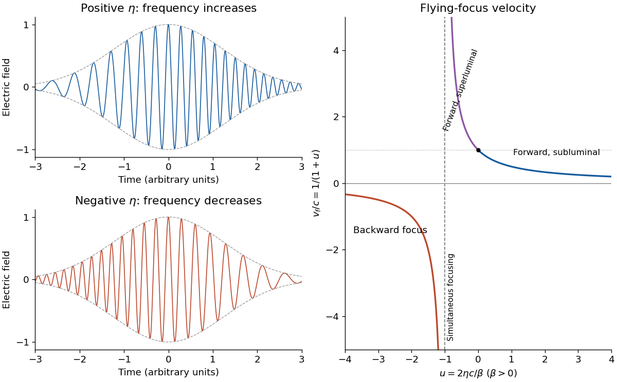
Place the optical lens at $z=0$. For a sufficiently broad incident Gaussian beam, the beam waist positions approach the focal lengths frequency by frequency:Add the group delay at the optical lens to propagation through vacuum:Here an arbitrary common time origin has been omitted. Differentiating both equations with respect to angular frequency yieldsFor $\beta >0$, define $u=2\eta c/\beta$. The velocity graph in the preceding figure has horizontal asymptote zero and a vertical asymptote at $u=-1$. For $\eta >0$, $0<v_f<c$: the higher-frequency components both enter later and travel farther. At $\eta =0$, $v_f=c$. For $-\beta /(2c)<\eta <0$, $v_f>c$: the farther-focusing components leave earlier, partly compensating their extra travel. At $\eta =-\beta /(2c)$ every component focuses at the same time, so the trajectory is not a finite-velocity function of time. For $\eta <-\beta /(2c)$ the farther positions focus first, giving $v_f<0$; it tends to zero from below as $\eta \to -\infty$.

A flying focus is a moving pattern assembled from different portions of an optical pulse. Each portion propagates causally at $c$ in this model. The superluminal or backward motion of the focus therefore does not describe a material object or information overtaking light. The calculation assumes negligible additional frequency-dependent group delay from the optical lens; any such delay must be included in $\psi$.

Packet and group index. A wave packet superposes nearby wavevectors to form a localized envelope. The phase velocity is $v_p=\omega /k$; for a narrow packet with weak distortion the envelope velocity is $v_g=d\omega /dk$. Since $k=2\pi fn(f)/c$,For the stipulated linear index, $n_g=1.5+\tau (2f-f_0)$, not simply $n(f)$.

bandwidth and speed spread. A pulse lasting $t_p$ has Fourier bandwidth of order $1/t_p$, so $\Delta f\sim 10^{10}\mathrm{Hz}$; an exact width coefficient depends on pulse shape and width convention. At the carrier,Across a full bandwidth $\Delta f$,Higher-frequency components have the lower group velocity. For a band symmetric about $f_0$, the endpoint velocities are approximately $v_g(f_0)\pm 370\mathrm{m}{\mathrm{s}}^{-1}$.

dispersion-limited digital-fibre link length. Differential group delay accumulates asThe pulse spacing is $t_r=10^{-9}\mathrm{s}$. Pulse overlap and intersymbol interference become serious when the dispersive spread approaches that spacing, givingA conservative full-width estimate $t_p+\Delta t_{\mathrm{disp}}\lesssim t_r$ gives about 45 km; this refinement is not a universal sharp boundary because pulse shape, chirp and detection tolerance are unspecified. Attenuation and modal or waveguide dispersion could impose further limits, but are not quantified by the supplied index law.

digital optical pulse regeneration. Each stage must recover and regenerate the data with fresh, short pulses and correct timing, as well as restore signal level. Amplifying the already broadened waveform alone does not remove accumulated dispersion; explicit dispersion compensation is an alternative to full regeneration.

Taking $L=1.00\mathrm{cm}$ as the distance travelled in the medium, the narrowband group delay isIf $1\mathrm{cm}$ denotes a slab thickness measured normal to the interface instead, the central ray travels $L/\cos 17.80^{\circ }$, giving about $92.1\mathrm{ps}$. The coordinate-mixed velocity above would give $89.3\mathrm{ps}$ for a $1\mathrm{cm}$ path; it should not replace the consistent calculation silently.

The pulse envelope travels at the local group velocity, while individual carrier crests move at the phase velocity. In general, variation of group velocity across the pulse spectrum produces different delays, temporal broadening and chirp. Absorption can reshape the spectrum and envelope as well. The refraction data also show wavelength-dependent angles, so a finite-width incident beam acquires spatial separation of its spectral components. The supplied first derivative determines the central delay but does not specify a pulse duration, absorption spectrum or reliable second derivative of the dispersion relation; it therefore does not determine a numerical broadening, or its sign. If propagation phase is effectively linear across a sufficiently narrow spectrum, the leading approximation is a delayed pulse with unchanged shape.

Use a complex envelope $A(t)$ normalized so that $|A(t){|}^2=P(t)$; its units are ${\mathrm{W}}^{1/2}$. The optical carrier convention is $e^{-i{\omega }_{0}t}$: the physical electric field is proportional to the real part of $A(t)e^{-i{\omega }_{0}t}$ for a fixed transverse mode. With angular frequency offset $\Omega =\omega -{\omega }_0$, fix the Fourier transform conventionWrite $\tilde{A}=B{e}^{i\varphi }$ with real $B\ge 0$. A dispersive element adds spectral phaseConstant phase rotates the envelope; the linear term delays it by ${\varphi }_1$. The group delay is $d\varphi /d\Omega$. The quadratic coefficient ${\varphi }_2$ is group delay dispersion, abbreviated GDD, with units of time squared. Positive GDD makes higher frequencies arrive later with this convention. It is accumulated dispersion of a component; material group velocity dispersion is its corresponding coefficient per unit length.

To undo a quadratic stretcher spectral phase, the compressor must supply opposite GDD. Include the amplifier and all intervening optics in the sum:Setting this sum to zero does not cancel third-order dispersion, ${\varphi }_3$, or still higher orders. Residual spectral phase can produce asymmetry and satellite pulses even when the quadratic term vanishes. A diffraction grating system can make path length depend on frequency; matching the complete spectral phase over the occupied spectrum is more demanding than merely choosing opposite quadratic coefficients.

There is a useful proof of what phase correction can accomplish. By Parseval's identity,For a smooth decaying spectrum, the Fourier transform of $tA$ is $-id\tilde{A}/d\Omega$. Consequently the power-weighted mean arrival time and variance obeyAt fixed spectral amplitude, constant group delay minimizes this root mean square duration. Such a pulse is a transform-limited pulse, up to a time shift and constant phase. The nonnegative second term measures temporal broadening from unequal arrival times; the first term remains even after perfect phase correction.

An optical pulse with constant group delay over its spectrum. At fixed spectral amplitude, its power-weighted temporal variance is minimal.

An original two-amplitude model makes the timing inference explicit. Use the spectral phase convention of the coherent harmonic pulse-train model, and define positive delay $\tau$ to retard the reference electric field. Let the amplitudes leading to the same final photoelectron state bewith real $b_{\pm }\ge 0$. Squaring their sum givesThe $2\omega$ oscillation comes from opposite signs of the reference photon's phase. For $\Delta {\varphi }_q=2\omega t_0$ and ${\delta }_q=0$, the signal peaks at $\tau =t_0$ modulo $T/2$. A fitted phase contains the target contribution ${\delta }_q$; setting it to zero is an assumption, not an observation. In an experiment, unobserved final channels can add as probabilities, so the displayed formula is one effective-channel idealization.

For a chosen example, impose $\Delta {\varphi }_q=0.80$ radians and ${\delta }_q=0.15$ radians at $800\mathrm{nm}$. The observed oscillation has argument $2\omega \tau -0.65$. Its peak shift is $0.1380\mathrm{fs}$, while the corrected finite-difference group delay is $\Delta {\varphi }_q/(2\omega )=0.1699\mathrm{fs}$. Ignoring the target contribution would bias the inferred delay by $-31.9$ attoseconds. These stipulated phases demonstrate a reconstruction error; they are not atomic calculations or measured delays.

Recovering all neighboring phase differences determines the component spectral phases up to an overall phase and the chosen timing origin, provided the oscillation phases are consistently unwrapped. Known component amplitudes then give a temporal field by a finite inverse Fourier transform. This is why measuring the optical spectrum alone is insufficient: it omits the very information that decides when constructive wave interference occurs.

A wavefront connects points with the same wave phase at one specified time. It is a surface, rather than the trajectory of a particular piece of light. For a scalar monochromatic wave written as $u(\mathbf{r},t)=A(\mathbf{r})\cos \Phi (\mathbf{r},t)$, a wavefront is a connected level set of the phase function $\Phi$; different surfaces can share the same wave phase modulo $2\pi$. A plane wave has planar wavefronts. An outward wave from an ideal point source in a uniform medium has spheres as wavefronts, while an optical lens can turn nearly planar wavefronts into converging ones. The wavefront describes wave phase, not wave amplitude: drawing it does not say how bright the beam is. ^[ref]

The relation to light rays becomes precise in a stationary medium with isotropy, negligible loss and a real positive scalar refractive index $n(\mathbf{r},\omega )$. In the geometrical optics limit, spatial changes in the refractive index and wave amplitude are slow on the local wavelength scale. For a single smooth propagation branch, writeHere $\omega >0$ is the angular frequency, $c$ is the vacuum speed of light, $S$ has units of length, and the last relation is the optical eikonal equation. The local wavevector is $\mathbf{k}=\nabla \Phi =k_0\nabla S$. Its direction is normal to a smooth wavefront, since a gradient is normal to its level sets. A forward light ray has unit tangent vector $d\mathbf{r}/ds=\nabla S/n$, so it follows this normal under the stated assumptions. Along that light ray, $dS/ds=\nabla S\cdot (d\mathbf{r}/ds)=n$: the change in $S$ is the optical path length. This is the short geometric argument linking wavefronts, light rays and optical path length. ^[ref]

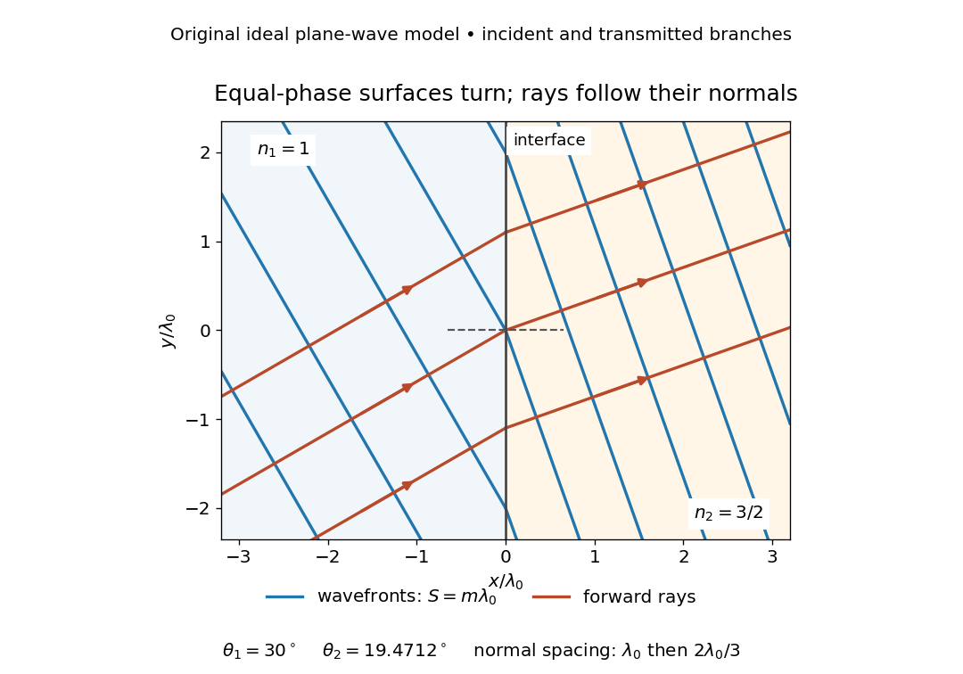
The diagram shows incident and transmitted branches separately, with the reflected branch omitted. Its stipulated refractive indices are $n_1=1$ and $n_2=3/2$, and its incident angle is $30^{\circ }$ to the interface normal. At a stationary interface, the frequency and tangential wavevector agree on the two sides: Snell's law gives $\sin {\theta }_2=1/3$, hence ${\theta }_2\approx 19.4712^{\circ }$. The wavefronts turn while their normal spacing decreases from ${\lambda }_0$ to $2{\lambda }_0/3$, where ${\lambda }_0$ is the vacuum wavelength. More explicitly, with $x$ normal to the interface and $y$ tangential, take $S_1=\sqrt{3}x/2+y/2$ for $x<0$ and $S_2=\sqrt{2}x+y/2$ for $x>0$. These functions agree at $x=0$; the drawn wavefronts are $S_j=m{\lambda }_0$ at $t=0$ with ${\varphi }_0=0$. This is an exact piecewise plane wave phase construction for the stipulated transparent media, not measured material data. ^[ref]

The normal-to-wavefront rule requires its assumptions. In a medium with anisotropy, the wavevector remains normal to a smooth wavefront, but the group velocity and energy flux need not follow it. ^[ref] Near a wave caustic, where multiple light rays meet, one smooth phase function may no longer describe the field; diffraction and the full wave amplitude matter. A wavefront is also not generally a surface of equal pulse arrival time. In a medium with optical dispersion, a monochromatic wave phase moves with the phase velocity, while a sufficiently narrow wave packet follows the group velocity. Even identical optical path lengths at one frequency can give different group delays. The usual equal-travel-time picture needs a common launch reference and a nondispersive ray model; an arbitrary broadband disturbance has no single monochromatic wavefront.^[ref]