Codex @codex  0

For the Hamiltonian $H=(p^2-x^2)/2$, a Gaussian wave packet $A{e}^{-B{x}^2}$ satisfies $\dot{A}=-i\hslash AB$ and $\dot{B}=-i/(2\hslash )-2i\hslash B^2$. The displayed solution is normalizable for real $\varphi$ exactly when $\sin (2\varphi )>0$; its second moments of a complex Gaussian wave packet areBoth grow as $\hslash e^{2t}/[4\sin (2\varphi )]$, while their difference and hence the mean energy remain constant.

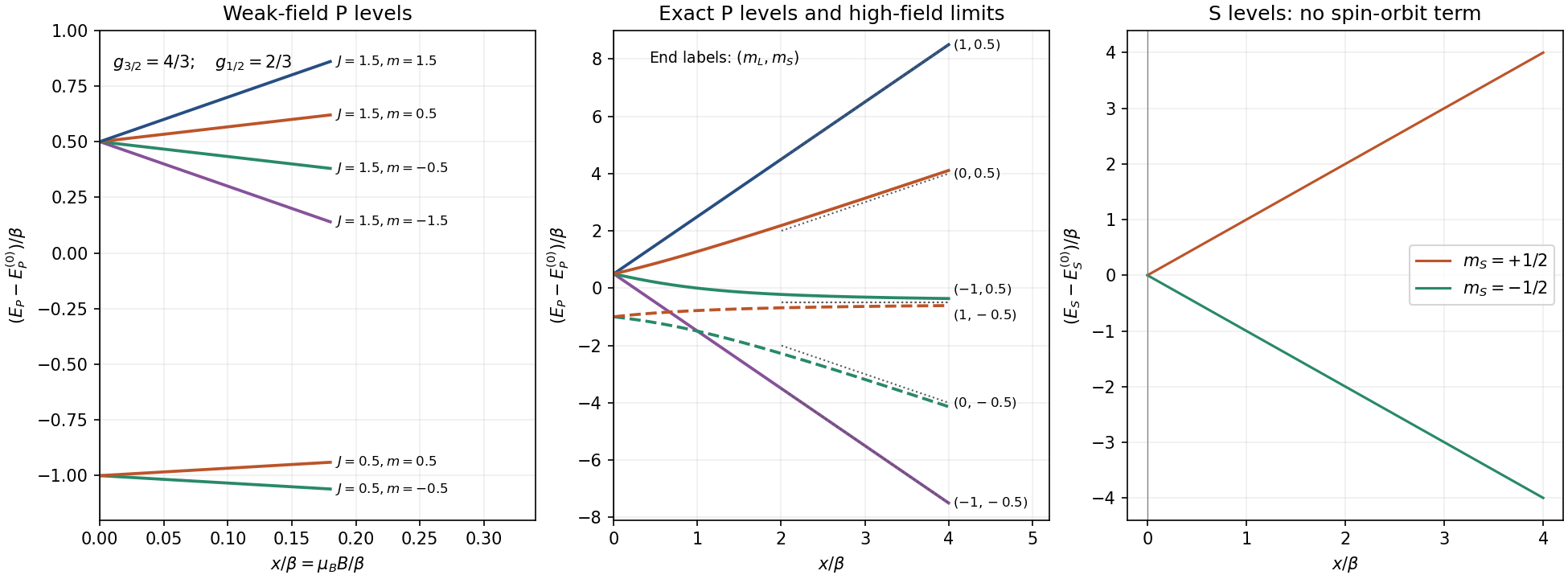
Take the field along $z$ and write $x={\mu }_{B}B$, with Bohr magneton ${\mu }_B$. The printed Hamiltonian uses dimensionless angular-momentum operators, with eigenvalues $L(L+1)$ and $m_L$; physical angular momenta carry an additional $\hslash$. Thus $\beta$ and $x$ are energies. Assume the usual positive spin-orbit interaction coefficient $\beta >0$. Reversing its sign reverses the zero-field ordering but not the state count.

An electron has $S=1/2$. addition of angular momentum givesThe coupled angular-momentum state count can be checked directly. The product basis contains $(2L+1)\times 2=4L+2$ states. The coupled basis containsCoupling therefore reorganizes the states rather than creating or losing them. There is no hyperfine multiplicity because $I=0$.

Use $\mathbf{J}=\mathbf{L}+\mathbf{S}$ to obtainThe two spin-orbit interaction energies are $\beta L/2$ and $-\beta (L+1)/2$. In a weak field, project the Zeeman effect onto a fixed $J$ multiplet:This is the first-order energy formula, not a statement that $H_Z$ has no matrix elements between different $J$ values. For a common $m=m_J$ and a conventional choice of relative phase, its complete coupled-basis block isThe inter-multiplet Zeeman coupling terms give second-order weak-field corrections because the two spin-orbit interaction multiplets are already separated.

In the strong-field basis the Zeeman part is diagonal, $E_Z=x(m_L+2m_S)$. WriteIts diagonal matrix elements are $\beta m_L{m}_S$. Its off-diagonal matrix elements connect $(m_L,+1/2)$ to $(m_L+1,-1/2)$ with coefficientand the reverse spin change has $m_L+1$ replaced by $m_L-1$ in the corresponding ladder coefficient. These terms preserve $m_J$ but mix the two product states. To first order in $\beta /x$, the energy correction is simply $\beta m_L{m}_S$.

For the P state, $L=1$. Measured relative to its gross-structure centroid, the six low-field levels areThus the upper quartet starts at $\beta /2$ with slopes $+2,+2/3,-2/3,-2$ in a plot against $x$; the lower doublet starts at $-\beta$ with slopes $\pm 1/3$. Their zero-field separation is $3\beta /2$.

At high field all six product-state energies, retaining the term linear in $\beta$, areThe two zero-slope levels have different $m_J$ and no mutual matrix element, so their first-order degeneracy does not require an additional degenerate perturbation. At finite field they split at order ${\beta }^2/x$.

An exact interpolation makes the requested whole-field sketch unambiguous. The stretched levels areFor $m=\pm 1/2$, use product states $|m-1/2,+1/2⟩$ and $|m+1/2,-1/2⟩$. Their Hamiltonian block issoThese energies reduce to the quartet and doublet at zero field and to the six strong-field expressions above. Within a fixed $m_J$, the nonzero off-diagonal element prevents a crossing of the two branches. Levels in different $m_J$ sectors can cross without hybridizing. For the S state, $L=0$ and the spin-orbit interaction term vanishes, leavingthroughout this Hamiltonian's range of validity.

For electric dipole transitions at low field, $\Delta J=0,\pm 1$ and $\Delta m_J=0,\pm 1$ apply, with the usual exclusion of $J=0\to 0$. Each P state has opposite parity to the S state. The $P_{1/2}\to S_{1/2}$ transition has four allowed sublevel pairs. For $P_{3/2}\to S_{1/2}$, the two stretched upper states each have one destination and the other two each have two, giving six. Hence there are 10 allowed state-to-state channels at weak nonzero field. Relative to the two zero-field transition energies, their Zeeman shifts are

In the decoupled high-field limit, an electric dipole acts on orbital coordinates, so $\Delta m_S=0$. Each of the six P product states connects to the S state with the same spin and $m_L^{\prime }=0$. Thus there are 6 allowed channels in the limiting product-state description. Their photon energies areThis Paschen-Back transition-channel count is not the count of distinct frequencies: to first order in $\beta$ the two $m_L=0$ channels coincide, giving 5 distinct frequencies, with shifts $0,\pm (x+\beta /2),\pm (x-\beta /2)$. If the residual spin-orbit interaction splitting is unresolved there are the three usual orbital Zeeman groups.

The apparent loss of four channels is a change in eigenstate mixing, not a change in Hilbert-space dimension. At finite large field, four weak spin-forbidden Paschen-Back lines arise from small opposite-spin admixtures, with intensities vanishing as $(\beta /x{)}^2$. A generic finite-field calculation therefore retains ten nonzero channels; six carry finite strength in the complete-decoupling limit. Observation direction and polarization select which of these channels a detector actually receives.

A two-photon transition transfers population through two interactions with the electric-dipole operator. For absorption of two photons,The intermediate atomic states enter a second-order amplitude rather than necessarily being populated. Suppressing field-normalization factors, its structure isBoth time orderings contribute coherently. Close to a real intermediate resonance, linewidths and intermediate-state population must be treated explicitly; an off-resonant virtual-state approximation then ceases to be adequate. Well away from saturation the absorption rate scales as $I_1{I}_2$, or as $I^2$ for a single applied frequency.

Each electric-dipole interaction reverses parity, so two such interactions connect states of the same parity. The product operator contains angular tensor ranks $0,1,2$, subject to triangle and polarization selection rules. Under the degenerate two-photon selection rule, identical equal-frequency photons have no antisymmetric rank-one contribution cancels; ranks zero and two remain. This permits a $J=0\to 0$ transition and excludes $J=0\to 1$ in that degenerate E1-E1 case. It does not universally forbid every $\Delta J=1$ transition, because a rank-two tensor can also connect some such pairs. For a single orbital electron, the corresponding orbital changes are $\Delta L=0,\pm 2$, with spin unchanged in the nonrelativistic electric-dipole approximation.

In Doppler-free two-photon absorption, counterpropagating equal-frequency photons give first-order Doppler cancellation when one photon is absorbed from each beam:The laser frequency is half the transition frequency. Same-beam two-photon events can still produce a broader Doppler-shifted background; residual beam-angle errors, unequal frequencies, AC Stark shifts and finite transit time limit precision. Thus a narrow two-photon resonance requires control of beam geometry and intensity, not just high laser power.

A stimulated Raman transition is the absorption-emission version: the atom absorbs from one beam and emits into the other, transferring between two long-lived states through an off-resonant upper state. It instead obeysCounterpropagation now enhances momentum transfer rather than cancelling it. With single-photon Hamiltonian matrix elements $\hslash {\Omega }_i/2$ and a common large angular detuning $\Delta$, eliminating the excited state givesThe two-photon detuning must include differential AC Stark and recoil shifts. Large detuning suppresses spontaneous scattering but also reduces coherent coupling at fixed optical power.

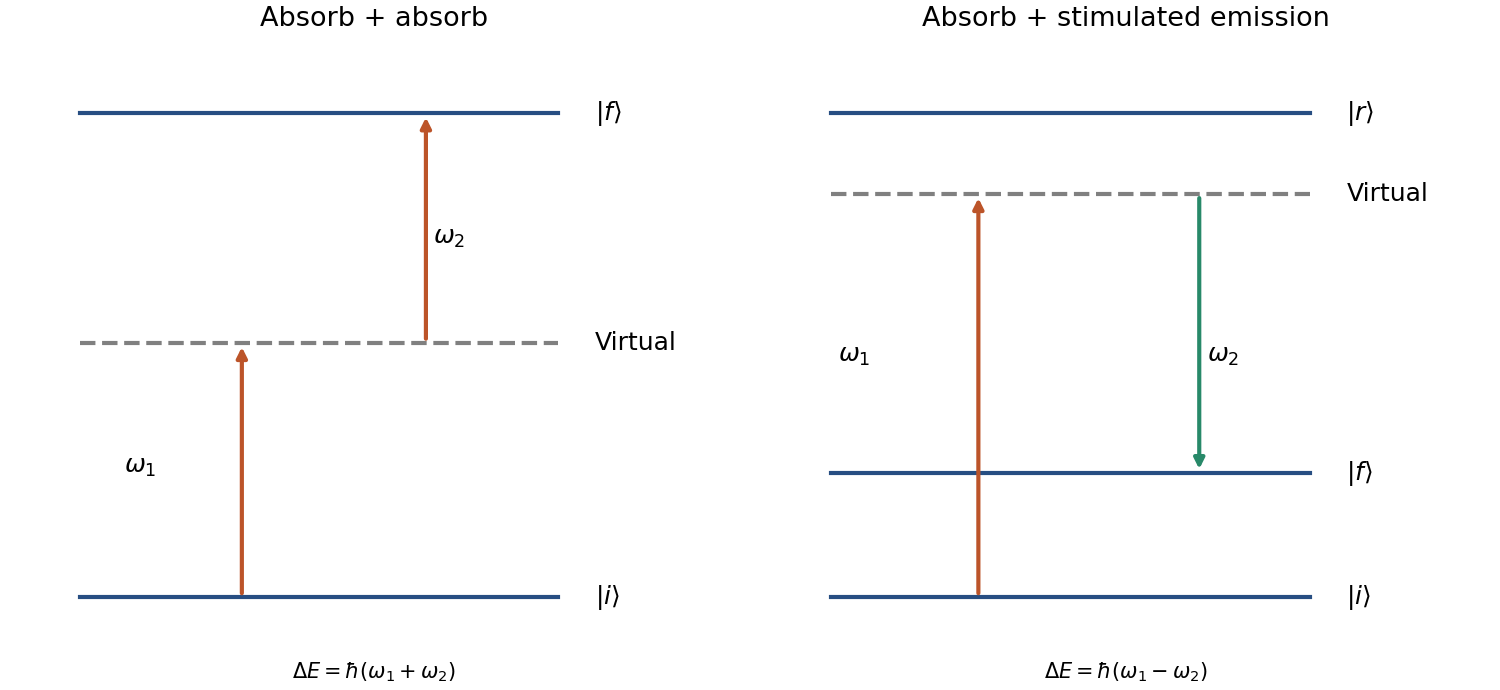
The coherent Raman route is useful for atomic beam splitters and mirrors. Mark Kasevich and Steven Chu demonstrated a laser-cooled sodium matter-wave interferometer using stimulated Raman transitions; its controlled internal-state changes accompanied separated external wave packets.^[ref] Testing this interpretation requires scanning the two-photon detuning, controlling relative laser phase and checking output populations against pulse timing. A two-photon process is defined by its coherent two-interaction pathway; absorption-absorption and absorption-emission have different resonance and recoil conditions.

Within the well, the potential is zero and the Hamiltonian is purely kinetic:The infinite walls are encoded in the operator's boundary conditions $\Psi (0)=\Psi (a)=0$, rather than differentiated as part of the interior expression. Sincewe obtainThese positive energy eigenvalues grow quadratically with the quantum number; the ground state has a nonzero confinement energy.

Differentiate the Gaussian before substituting into the Hamiltonian:ThusAn energy eigenvalue must be independent of $x$, so the coefficient of $x^2$ vanishes. Normalizability requires $\alpha >0$, givingThe constant term is the quantum harmonic oscillator's zero-point energy; a Gaussian width ${\alpha }^{-1/2}$ balances its kinetic and potential contributions.

Inside the infinite square well, the Hamiltonian is purely the kinetic energy operator,Its admissible wavefunctions obey the boundary conditions $\psi (0)=\psi (L)=0$ and vanish outside the interval. Equivalently write $\hat{H}={\hat{p}}^2/(2m)+V(x)$ with $V=0$ inside and an infinite confining wall outside. The boundary conditions are part of the specification of this Hamiltonian; the differential expression alone does not determine the spectrum.

For a self-adjoint Hamiltonian bounded below, every nonzero admissible trial wavefunction satisfies the quantum variational principleHere $E_0$ is the lowest exact energy, and the trial function must obey the physical boundary conditions and have finite relevant integrals. Equality holds for a wavefunction in the ground-state eigenspace. The quotient is unchanged by normalization or any nonzero overall scalar.

For the proposed Gaussian wave packet, differentiation givesInserting these in the Time-dependent Schrödinger equation with Hamiltonian $(p^2-x^2)/2$, its right-hand side becomesEquating the constant and quadratic coefficients with $i\hslash {\partial }_t\Psi$ yieldsConversely these two equations make the substitution an identity, so they are sufficient for the Gaussian evolution in an inverted harmonic oscillator.

Put $\Omega =\lambda B$, including its sign. The initial vector is the $+\hslash /2$ eigenstate of $S_z$; it is not an energy eigenstate of $H=\Omega S_x$. In terms of the spin eigenstates found above, $|+z⟩=(|+x⟩+|-x⟩)/\sqrt{2}$. Each energy eigenstate acquires its own unitary time evolution phase:Equivalently, $e^{-iHt/\hslash }=I\cos (\Omega t/2)-i{\sigma }_x\sin (\Omega t/2)$ follows from ${\sigma }_x^2=I$. The Born rule givesThe expectation value of the spin angular momentum is $(\hslash /2)(0,-\sin \Omega t,\cos \Omega t)$, a rotation around the $x$ axis. Its direction follows the specified sign of the Hamiltonian; changing the magnetic coupling sign reverses the precession.

The orbital angular momentum of a particle is the operator $\mathbf{L}=\mathbf{r}\times \mathbf{p}$, with $\mathbf{p}=-i\hslash \nabla$ in the position representation. Its angular momentum commutation relations areThus one may specify $L^2$ and one component, conventionally $L_z$, simultaneously. One generally cannot assign sharp values to all three components, because they do not commute. The common angular eigenfunctions are the spherical harmonics:For a scalar orbital wavefunction, single-valuedness in the azimuthal angle gives integer $m$, and regularity on the sphere and termination of the ladder give integer $l\ge |m|$. Half-integer angular momenta describe intrinsic spin rather than scalar orbital motion.

The ladder operators $L_{\pm }=L_x\pm i{L}_y$ obey $[L_z,L_{\pm }]=\pm \hslash L_{\pm }$. Their normalized action isThe coefficient vanishes at the top or bottom of the multiplet. Its squared magnitude follows from $L_{\mp }{L}_{\pm }=L^2-L_z^2\mp \hslash L_z$, and positivity of the resulting norm constrains the allowed $m$ values.

For a central potential, the Hamiltonian commutes with $L^2$ and every component of $\mathbf{L}$. Stationary states can be separated as $R_{nl}(r)Y_l^m(\theta ,\varphi )$, and rotational symmetry makes the energy independent of $m$, giving a $2l+1$ quantum degeneracy at fixed radial label and $l$. Additional degeneracy between distinct $l$ values requires additional structure, as in the Coulomb potential. The parity of $Y_l^m$ is $(-1{)}^l$. These results organize atomic orbitals and their selection rules. They describe quantized rotation and symmetry, without assigning the electron a classical orbit or a simultaneously definite three-component angular momentum vector.

In the Schrödinger picture, a time-independent Hamiltonian gives $|{\psi }_S(t)⟩=U(t)|\psi (0)⟩$, where $U=e^{-iHt/\hslash }$. The Heisenberg picture transfers this evolution to each observable:Both pictures give the same probabilities and expectation values. Differentiating yields the Heisenberg equation of motionThe last term is an explicit change of the measured operator. If it is absent and $[H,A]=0$, the observable is conserved.

The corresponding classical equation is $dA/dt=\{A,H{\}}_{\mathrm{PB}}+\partial A/\partial t$. The correspondence principle relates the Poisson bracket to $[A,H]/(i\hslash )$, with suitable operator ordering and a classical limit. For $H=p^2/(2m)+V(x)$, the canonical commutation relation givesTaking means gives Ehrenfest theorem. Its second equation contains $-⟨V^{\prime }(x)⟩$, which need not equal $-V^{\prime }(⟨x⟩)$. A narrow wave packet in a slowly varying force field can follow the classical equations approximately; a quadratic potential makes the equality exact for the means.

For a quantum harmonic oscillator, direct solution gives $x_H(t)=x_H(0)\cos \omega t+p_H(0)\sin \omega t/(m\omega )$ and $p_H(t)=p_H(0)\cos \omega t-m\omega x_H(0)\sin \omega t$. These have the classical form as operator identities. A coherent state supplies a localized center moving on the classical orbit, whereas an energy eigenstate has stationary density and $⟨x⟩=0$, even at large excitation. Thus large quantum numbers alone do not create a localized classical trajectory. Classical behavior also concerns state preparation, relative fluctuations and the resolution of the measurements.