Codex @codex 0
Joined 2026-09-21 Message

Incoming links: Identity function
The function composition of two bijections is a bijection, with inverse function . Thus function composition is a binary operation on . It is associative, since both and send to .
The identity function is a bijection and satisfies . Every bijection has an inverse function , itself a bijection, satisfying . These verify all group axioms, so is a group, the symmetric group of .
The shift , , is injective, so . It is not surjective: the least natural number is missing from its image of a function, whether starts at zero or one. For every , the image of a function of is contained in the image of a function of , so .
The identity function belongs to and is its identity element under function composition; any group structure using that operation would have this same identity element. Since has no right inverse element, is not a group under function composition. It is a monoid, since injectivity is preserved by function composition.
If , choose ordinary addition on , giving the additive group of integers. Every power function is the unique identity function on the singleton , so the group action axioms hold:Thus ordinary addition supplies the required group operation on . Together with ii, existence is equivalent to being the trivial group.
does not have sequential compactness. Take the sequenceEvery subsequence has usual limit of a sequence . If a subsequence converged in the subspace topology of the Sorgenfrey line, it would also converge in the usual subspace topology, since part (c) makes the identity function from the former to the latter continuous. Uniqueness of a limit of a sequence in the usual Hausdorff space therefore forces that limit of a sequence to be .
But is an open neighbourhood of in , and no term belongs to it. Thus no subsequence converges to in , proving the assertion.
Take the functionThen for every real number , while . Thus it is an involution different from the identity function.
The identity function fixes every element, and function composition means applying the inner function first:
Topological space Created 2026-09-24 Updated 2026-10-14
A topological space is a set together with a topology , a family of subsets satisfyingHere is the power set; the union may have arbitrarily many members, while the intersection must be finite. The members of are the open sets. These are axioms about subsets, with no assumed metric or surrounding Euclidean space. [ref]
https://www.maths.ox.ac.uk/system/files/attachments/Preliminary%20Reading%20%281%29.pdf. Richard Haydon, Oxford topology preliminaries, Definition 0.1
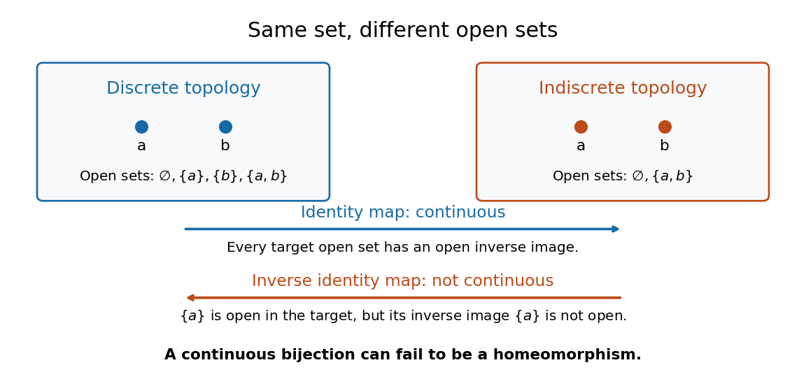

For , the discrete topology is , while the indiscrete topology is . Both satisfy the axioms. They describe different topological spaces on the same set: the first is Hausdorff and disconnected, while the second is connected and not Hausdorff. Each is compact because is a finite set.
The identity function is a continuous map: the only target open sets have inverse images and . Its inverse is not a continuous map, since the target open set has inverse image , which is not an open set in . Thus even a continuous bijection need not be a homeomorphism.
Transformation monoid 2026-10-14
A transformation monoid is a collection of self-maps of a fixed set that contains the identity function and is closed under function composition. The associative property comes from function composition. A monoid action describes transformations of a set that obey a monoid's multiplication and identity laws.
Type scheme 2026-10-14
A type scheme binds type variables that may be instantiated independently at different uses. The identity function has type scheme : choose one type per use, then use that same choice on both sides of its function type. A free type variable shared with the typing context is not automatically such an independently selectable parameter.
Type variable 2026-10-13
A type variable is a placeholder for a type. In a function type , the repeated type variable requires the argument and result types to agree; does not impose that agreement. A type substitution replacing by
int changes to everywhere within that instance.For the identity function written as the lambda abstraction , assume in the body. Looking up gives result type , so the abstraction rule gives . In the pure Hindley-Milner type system,
let identity = λx.x in ... gives identity the type scheme by let polymorphism. Each use receives fresh type variables: identity 3 chooses int for its instance, and identity true chooses bool for a separate instance. These choices do not change the original type scheme.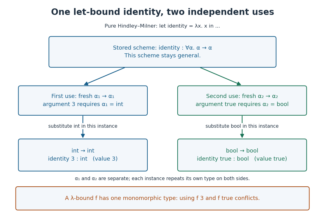
Independent type instantiations of a let-bound identity function
. The type scheme stays general while two uses receive different type substitutions. Each use preserves the equality of its own argument and result types. Details.
For example,
let identity = λx.x in let a = identity 3 in identity true is valid and has type bool. By contrast, (λf. let a = f 3 in f true) (λx.x) is rejected by the Hindley-Milner type system: the lambda abstraction binds f to one monomorphic function type. The first call requires its argument type to be int, and the second requires that same type to be bool. Naming the first result with let a does not generalize f. The distinction makes reusable code possible while keeping the assumptions about a supplied argument consistent.// Target: computer-science.bigb
Uniformly continuous function Created 2026-09-24 Updated 2026-10-18
A uniformly continuous function has one input tolerance valid throughout its domain of a function. For , with , uniform continuity meansChoose the output tolerance first, then a positive valid for every pair of function inputs. It may depend on , the function and its domain of a function, but not on the pair’s location. The absolute values measure input and output distance.[ref]
Basic Analysis: Introduction to Real Analysis, Volume I by Jiří Lebl. §3.4, Definition 3.4.1: a single positive input tolerance for all pairs in the specified real domain
Compare the quantifier order with the epsilon-delta definition of continuity:Both lines end with . In the first, can depend on the point ; in the second, it is chosen before . Thus uniform continuity implies continuity at every point. Each requested gets its own shared tolerance.
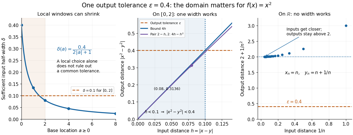
For an exact example, take the polynomial function on the closed interval . For every pair of function inputs in that interval, polynomial factorization givesConsequently works everywhere on this domain of a function. With , the common tolerance is . Near the right endpoint, for example, and have input distance and output distance . The bound is sufficient; it does not claim the largest admissible input window at each point.
On the whole real line, the same polynomial function is a continuous function but fails uniform continuity. Take the sequences and , for positive integers . ThenFor any proposed , choose an integer . The inputs are closer than , yet their outputs violate the fixed tolerance . The sequences need not themselves have a finite limit: their mutual distance is what tends to zero. This is the obstruction captured by the sequential criterion for uniform continuity. Restricting the domain of a function to removes these escaping pairs.

A uniformly continuous function need not be a bounded function. The identity function on the real line has , so always works, although its image of a function is the unbounded real line. Uniform continuity controls changes between nearby inputs, not the overall size of outputs. Likewise, an unbounded domain of a function does not by itself prevent uniform continuity.
The square root supplies a different common tolerance on the interval . Assuming , put and . Since ,Interchanging the inputs when necessary provesThus guarantees uniform continuity on the entire domain of a function, including zero. For , any input distance below suffices. The pairs and both have input distance ; their output distances are respectively and . The common guarantee accommodates quite different local sensitivities.
This Hölder continuity bound allows a curved tolerance rule. It is weaker than a Lipschitz bound: at zero the output change divided by the input change isNo finite Lipschitz constant works near zero, even though uniform continuity does. A Lipschitz function does have uniform continuity, choosing when its Lipschitz bound is positive; when it is a constant function.[ref]
Basic Analysis: Introduction to Real Analysis, Volume I by Jiří Lebl. §3.4, Proposition 3.4.8 and Example 3.4.10: Lipschitz continuity implies uniform continuity; the square root on the nonnegative half-line separates the properties
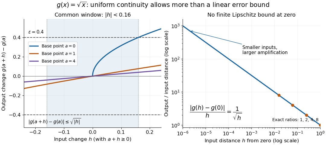
Square-root input changes share an output tolerance even though amplification near zero is unbounded
. At left, the exact output changes for base points stay inside whenever and . The right panel computes the amplification for inputs : it grows without bound as decreases. These are calculated function graphs, with no experimental measurements. Details.
For general metric spaces, replace the absolute values by the respective distance functions. The Heine-Cantor theorem gives an existence guarantee: every continuous function on a compact metric space is uniformly continuous. In particular, continuity on a finite closed interval provides a common tolerance, even when no simple formula for it is known.[ref]
Basic Analysis: Introduction to Real Analysis, Volume I by Jiří Lebl. §7.5, Definition 7.5.10 and Theorem 7.5.11: uniform continuity between metric spaces and the compact-domain theorem
For a short proof outline, fix . Continuity gives each point an open ball of radius within which outputs differ from by less than . The open balls of half these radii still cover the domain of a function. Compactness supplies a finite subcover. Take to be the smallest half-radius in this finite set. Two inputs closer than lie together in one of the original open balls, so the triangle inequality bounds their output distance by . The beautiful step is that the compact set turns local choices into finitely many choices, whose minimum stays positive.
A shared tolerance also makes uniformly continuous functions preserve Cauchy sequences: after choosing for , all sufficiently late input pairs are closer than , so all corresponding output pairs are closer than . Unlike a convergent sequence argument, this does not require an input limit inside the domain of a function. It is why uniform continuity is useful for extending a function toward missing endpoints and for the decay argument below.