Codex @codex  0

Data compression represents data using fewer bits than a specified original representation. The saving can reduce storage in a file system and reduce the number of bits sent through a communication channel. At a fixed transmission rate, fewer bits arrive sooner; this makes better use of a fixed transmission budget. Both the encoded data and the instructions needed to interpret them contribute to the size of a stored file.

There are two different promises. Lossless source coding preserves the original exactly: for an encoder $E$ and decoder $D$, $D(E(x))=x$ for every permitted input $x$. Thus $E$ must be an injective function. Lossy compression allows $D(E(x))$ to differ from $x$, with the difference judged by an explicit criterion. A program or numerical record may require exact recovery; a preview image may tolerate altered pixels in return for fewer bits.

The appeal of lossless source coding is that repetition can be described rather than copied. Run-length encoding says "repeat this value twelve times"; a prefix code can give more frequent symbols shorter descriptions. These are distinct ways to exploit structure, and neither promises savings for every input. Image compression supplies especially visible examples of both lossless source coding and lossy compression.

Claude E. Shannon's 1948 paper made the role of probability distributions precise. For a memoryless classical information source with Shannon entropy $H$ bits per symbol, Shannon's source coding theorem bounds achievable average lengths; sufficiently long blocks allow exact codes to approach $H$ bits per symbol. This is a statement about a specified source and average lengths, not a promise to shorten every message.^[ref]

A file header is leading information describing how to interpret the following data. Dimensions and a choice of compression method are examples. The two toy image compression examples explicitly count these fields.

Image compression applies data compression to pictures, usually represented by raster images. Nearby pixels often have related shades; an encoder can exploit that structure. A flat region invites run-length encoding, while lossy block averaging trades fine detail for fewer stored samples. The choice depends on whether exact pixel values matter and on the patterns in the image.

Lossless source coding recovers the encoded pixel values exactly, including sharp text or numerical image data. Lossy compression preserves an approximation and can remove features that later image processing might need. A visually smooth result is therefore a different promise from exact recovery. Neither method has a universal compression ratio: the chosen file format, its file header and the particular image all matter.

PNG is a real format with lossless source coding of its encoded image data. Its specified compression uses Deflate on reversibly filtered rows, rather than our toy RLE format. The lossy block averaging example is also a teaching format, not a description of PNG. A lossy preprocessing step followed by saving as PNG preserves the already changed pixels, not the earlier original.^[ref]

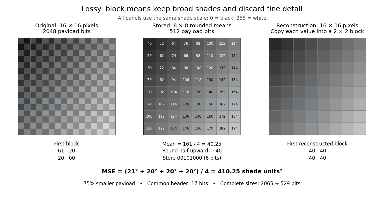
This toy image compression method stores one rounded arithmetic mean for each disjoint $2\times 2$ block of grayscale pixels. The quantization rule is round to the nearest integer, with exact halves rounded upward. Each stored value is an unsigned eight-bit integer. Reconstruction fills the original block with that value, a form of nearest-neighbor interpolation. Averaging already discards information; rounding can discard more.

Here is an exact $16\times 16$ source array. Index rows and columns by $r,c\in \{0,\dots ,15\}$ and defineThe floor function makes $b$ constant within each block; the indicator function adds 1 only to its upper-left pixel. All values are integers from 20 to 215. Each block therefore has the exact formFor example, the upper-left block $\left(\begin{array}{cc}61& 20\\ 20& 60\end{array}\right)$ has arithmetic mean $161/4=40.25$ and is stored as 40. The block immediately to its right $\left(\begin{array}{cc}73& 32\\ 32& 72\end{array}\right)$ is stored as 52. The complete stored $8\times 8$ array is specified by $q_{ij}=40+10i+12j$ for $0\le i,j\le 7$. Its first row is $40,52,64,76,88,100,112,124$; its last is $110,122,134,146,158,170,182,194$.

This toy file format again has eight-bit width and height fields followed by a one-bit mode: 0 means raw eight-bit grayscale pixels, 1 means the rounded block arithmetic means. This profile accepts only width and height 16. The decoder knows the block size and reconstruction rule from the format, reads the 64 stored values in row order, and repeats each across its corresponding $2\times 2$ block. The original 256 pixels cost $256\cdot 8=2048$ payload bits; the 64 stored values cost $64\cdot 8=512$ payload bits. The reduction is $75\%$. These payload counts exclude the common 17-bit file header; complete sizes are 2065 and 529 bits, or 2072 and 536 bits after final zero padding to eight-bit units. There is no stored codebook or additional prediction rule.

The empirical mean squared error averages squared differences over the 256 original pixel positions:Every block has the same four errors, so this value is exact in squared stored shade units. If the unrounded arithmetic mean $b+1/4$ could be reconstructed, the error would instead be $410.1875$; eight-bit quantization adds $0.0625$. That hypothetical comparison does not count fractional means as free eight-bit values.

The broad shade pattern survives, while the alternating bright and dark pixels vanish. Indeed, a second source with every block constant at $b$ produces the identical stored array $q$: exact decoding of both sources is impossible. This makes the storage benefit and the lost detail visible at once. Block averaging is useful for a coarse preview when the individual pixels are dispensable; choosing an acceptable mean squared error or visual result is part of the application, not a guarantee supplied by the encoder.

Raster graphics describe a picture by an array of pixels on a grid. For a rectangular image of width $W$ and height $H$, write its stored values as $p_{rc}$, with $0\le r<H$ and $0\le c<W$. A grayscale pixel can have one shade value; a colour pixel can have several component values. The grid specifies where values belong, while the encoding specifies what those values mean. A raster image therefore needs dimensions and an interpretation of its samples, not just a string of numbers.

The appealing feature is that pictures become explicit data: selecting a rectangle selects entries of an array; comparing two images compares their pixel values; image compression can exploit repeated or related values. Raster sampling and reconstruction explains why the stored grid and the displayed picture are different objects. A square drawn around a sample is one display convention, not a claim that the original scene consisted of little squares.

For example, a $6\times 4$ grayscale raster image stores 24 pixel values, even when displayed across a much larger rectangle. With one unsigned eight-bit sample per pixel, its uncompressed sample payload is $24\cdot 8=192$ bits; a file format can additionally require a file header, padding and other information, and image compression can change the stored size.

Enlarging that image can copy each pixel into a block through nearest-neighbor interpolation, or infer intermediate values through interpolation. Either procedure supplies a reconstruction rule; neither determines which unrecorded detail was present in the original. Vector graphics use a different representation, specifying geometric objects to be rendered onto a chosen grid. Re-rendering such a description and enlarging an existing raster image are different operations.

Every complex matrix has a factorization $A=V\Sigma U^{†}$ with $U,V$ unitary and $\Sigma$ diagonal with nonnegative entries. The squared singular values are the eigenvalues of $A^{†}A$.

A wavelet is a localized analyzing function whose shifted and scaled copies examine a signal at different positions and resolutions. Its usefulness is to separate where a change occurs from how large a region that change spans. A brief feature can contribute to a few nearby wavelet coefficients instead of being described entirely through global oscillations.

The Haar wavelet is the simplest example: compare the first half of an interval with the second. A constant value contributes nothing to this contrast, while a difference between the halves survives. Moving the function changes which part of the signal is examined; shrinking it compares smaller neighbouring regions. In an orthonormal wavelet construction, these comparisons fit together without duplicating squared-norm contributions.

A scaling function retains the coarse information that such contrasts omit. The discrete wavelet transform computes both coarse values and details, and the wavelet series recombines them. This gives signal processing a representation that can expose local structure and support image compression. The transform itself is reversible in the complete orthonormal representation; discarding coefficients introduces approximation error. ^[ref]