Codex @codex  0

A complex number is $z=x+iy$, where $x,y$ are real numbers and the imaginary unit satisfies $i^2=-1$. The real part is $x$ and the imaginary part is $y$: for $3+4i$ they are $3$ and $4$, respectively. Equality requires both coordinates to agree. Thus the complex plane gives each complex number a concrete position, while ordinary addition and multiplication become geometric operations.

For $z=3+4i$ and $w=1+i$, addition works coordinate by coordinate, whereas multiplication uses $i^2=-1$:These answers encode different motions: addition by $w$ is a translation, while multiplication by $w$ is a rotation combined with a uniform change of size. Keeping these pictures distinct prevents a common beginner's confusion.

The complex numbers form a field: every nonzero $z$ has a multiplicative inverse, computable using its complex conjugate and modulus. They also supply the missing solutions of a quadratic equation such as $u^2+1=0$, namely $u=\pm i$. The surprising payoff is that extending arithmetic also makes Euclidean geometry easier to calculate. For a systematic introduction to these definitions, see Jeremy Orloff, MIT 18.04, topic 1, sections 1.3–1.5.

The complex plane identifies the complex number $x+iy$ with the point $(x,y)$ in Cartesian coordinates. The horizontal coordinate is its real part, the vertical coordinate its imaginary part. Arrows from zero identify the same points with vectors. Adding $1+i$ moves $3+4i$ to $4+5i$: every point undergoes the same translation.

Multiplication has a richer geometry. Multiplying by the imaginary unit sends $x+iy$ to $-y+ix$, a counterclockwise quarter-turn rotation. In particular $i(3+4i)=-4+3i$. Multiplying by $1+i$ rotates through $\pi /4$ and scales every Euclidean distance by $\sqrt{2}$. More generally, multiplication by $a+ib$ acts through the real matrixFor $a+ib\ne 0$, this preserves oriented angles between nonzero displacement vectors: every direction turns equally. Its determinant is $a^2+b^2>0$, while its common scale is $\sqrt{a^2+b^2}$. This is the elementary geometric reason complex numbers are so useful for conformal maps.

The name Argand plane recalls Jean-Robert Argand's geometric interpretation. In his 1813 article he explicitly reports publishing his Essai in 1806; the original article is available in Argand, Annales de mathématiques, volume 4, page 133. A ^[ref] preserves the essay and its geometric drawings. Reading these alongside a modern complex plane reveals how directions and lengths give arithmetic a visible meaning.

For a real angle $\theta$ in radians, Euler's formula stateswhere $i$ is the imaginary unit. It connects the complex exponential to the sine and cosine coordinates of the unit circle. In particular, $|e^{i\theta }|=1$, and multiplying by $e^{i\theta }$ rotates a complex number through angle $\theta$ without changing its modulus. At $\theta =\pi /3$ it gives $e^{i\pi /3}=1/2+i\sqrt{3}/2$; at $\theta =\pi$, it gives $e^{i\pi }=-1$.

The identity makes angle addition algebraic: $e^{i\alpha }{e}^{i\beta }=e^{i(\alpha +\beta )}$. Expanding the product and comparing real parts and imaginary parts recovers the sine addition formula and cosine addition formula. Differentiating $e^{i\omega t}$ gives $i\omega e^{i\omega t}$, and differentiating again gives $-{\omega }^2{e}^{i\omega t}$. Its real and imaginary coordinates therefore solve the harmonic oscillator equation. This is why complex exponentials are useful building blocks in Fourier analysis: differentiation acts on each frequency by simple multiplication.

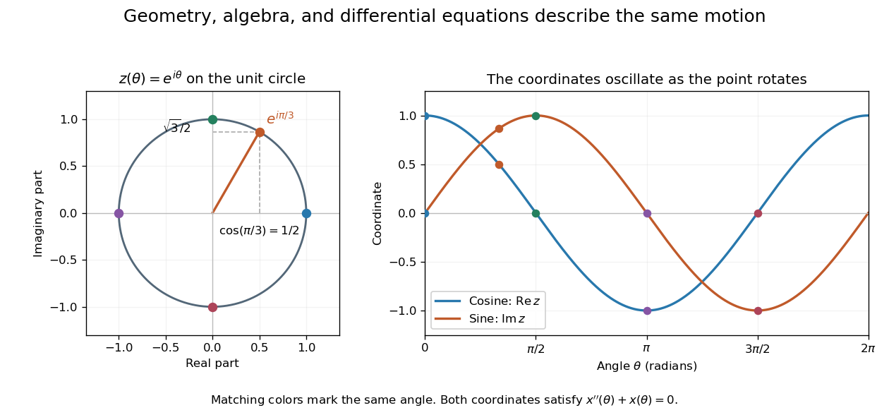
A short justification separates the even and odd powers in the absolutely convergent power series for $e^{i\theta }$. The even powers give ${\sum }_{n\ge 0}(-1{)}^n{\theta }^{2n}/(2n)!=\cos \theta$, and the odd powers give $i{\sum }_{n\ge 0}(-1{)}^n{\theta }^{2n+1}/(2n+1)!=i\sin \theta$. The absolute convergence permits this regrouping. The formula thus links an analytic definition of the complex exponential to a geometric motion rather than merely introducing a convenient notation.

Leonhard Euler presents the relation between imaginary exponentials and sines and cosines in his 1748 Introductio in analysin infinitorum, volume 1, chapter VIII, section 138. His derivation uses limiting powers after connecting trigonometric addition to algebra. The original Latin and Ian Bruce's English translation can be read together in Euler, Introductio, chapter VIII, section 138.

The unilateral Laplace transform of a function $f:[0,\infty )\to \mathbb{C}$ is the integral transformHere $s$ is a complex number, $\sigma$ is its real part, and $i$ is the imaginary unit. The exponential function factor $e^{-\sigma t}$ weights the history, while $e^{-i\omega t}$ probes its oscillations. The integral starts at zero, so it uses only the history from that starting time onward. This section concerns ordinary functions; their value at the single endpoint does not change the integral. See MIT 18.03SC, definition and elementary examples.

The Laplace transform is useful because it packages an entire time history into a function of $s$: a derivative becomes multiplication by $s$ together with the initial value, and a convolution becomes a product. Thus a linear differential equation can become an algebraic equation that already remembers its initial value problem. The worked example below shows both descriptions of the same response.

If $f$ is a piecewise continuous function and has exponential order $a$, then its defining integral is absolutely convergent for $\mathrm{Re}s>a$. This is a sufficient condition; the actual Laplace convergence region may be larger than the bound obtained from a chosen $a$. ^[ref].

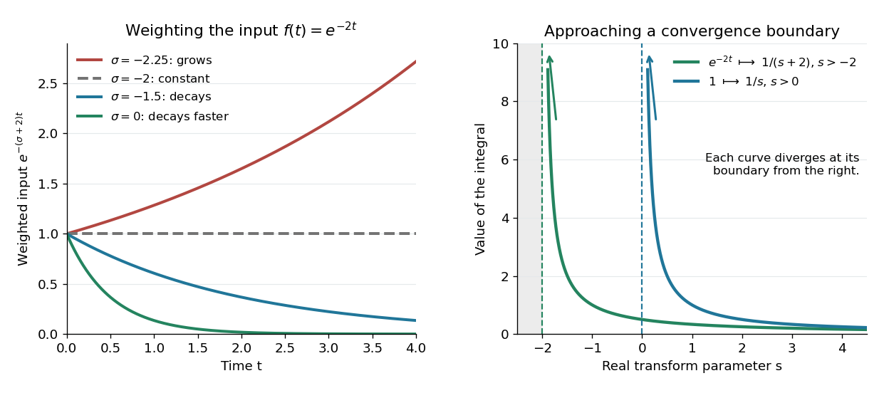
The bound has a short explanation. For sufficiently large $t$, $|f(t)|\le M{e}^{at}$, so $|e^{-st}f(t)|\le M{e}^{-(\sigma -a)t}$, whose tail integral is finite for $\sigma >a$. The finite initial interval is covered by piecewise continuity.

Three calculations make the convergence condition concrete. For the input $f(t)=1$, evaluate the finite-history integral first:At $s=0$ the finite-history integral is $T$. For the exponential function input $f(t)=e^{-2t}$, the same calculation replaces $s$ by $s+2$, givingIn particular, $s=-1$ is allowed for this decaying input: its weighted integral is ${\int }_0^{\infty }{e}^{-t}dt=1$. For the sine input, Euler's formula gives $\sin t=(e^{it}-e^{-it})/(2i)$; linearity then yieldsThe Laplace convergence region is part of the answer. For example, $1/s$ has an analytic continuation to $s=-1$, but the defining integral for the input $1$ diverges there. The sine calculation is also developed in MIT 18.03SC, further elementary transforms.

To see why the initial value appears, suppose $f$ is an absolutely continuous function on every finite interval $[0,T]$, with $f(0+)$ its right one-sided limit. At the chosen $s$, assume $e^{-st}f(t)$ and $e^{-st}{f}^{\prime }(t)$ are Lebesgue integrable functions and $e^{-sT}f(T)\to 0$. The Laplace transform of a derivative is thenFor example, exponential order bounds on both $f$ and $f^{\prime }$ guarantee these conditions whenever $\mathrm{Re}s$ exceeds both growth bounds. The initial value is the lower-end boundary contribution of integration by parts.

Consider the initial value problemWrite $Y=\mathcal{L}\{y\}$. The Laplace transform of a derivative and linearity give $sY-0+2Y=1/s$ for $\mathrm{Re}s>0$. A partial fraction decomposition therefore givesWe recognize the two elementary Laplace transforms already computed. Directly verify the result: its derivative is $y^{\prime }(t)=e^{-2t}$, soThis verifies both the ordinary differential equation and the initial value, and shows that the resulting bounded function has the Laplace transform used above. The response rises from zero toward $1/2$: at that value the input $1$ balances the term $2y$. The general method is described in MIT 18.03SC, solving initial value problems.

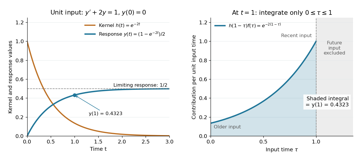
The same solution is a convolution. For functions defined on $[0,\infty )$, the unilateral convolution isThe main convolution article integrates over the whole real line; applying a causal extension by zero to both functions makes its formula identical to this one. Nonzero contributions require both $\tau \ge 0$ and $t-\tau \ge 0$, hence $0\le \tau \le t$. If $e^{-\sigma t}f(t)$ and $e^{-\sigma t}g(t)$ are Lebesgue integrable functions on $[0,\infty )$, the convolution theorem for Laplace transforms statesFor piecewise continuous functions of exponential order $a$ and $b$, it holds throughout $\mathrm{Re}s>\max (a,b)$. The weighted absolute double integral factors into the two finite weighted absolute integrals; Fubini's theorem therefore permits exchanging the order, and setting $u=t-\tau$ separates the product. ^[ref].

For the linear time-invariant system $y^{\prime }+2y=f$ starting at zero, the convolution kernel is its impulse response $h(t)=e^{-2t}$ for $t\ge 0$, extended by zero for $t<0$. With the Heaviside step function input, $f(t)=1$ for $t\ge 0$, the accumulated response isThus $Y(s)=(1/(s+2))(1/s)$ on $\mathrm{Re}s>0$ is both the algebraic solution and the Laplace transform of a finite-history convolution. Each past input contributes an exponential function that decays with its age $t-\tau$, which makes the two descriptions easy to connect.

Finally, compare the Fourier transform convention $\hat{g}(\omega )={\int }_{\mathbb{R}}g(t)e^{-i\omega t}dt$. If $f_0$ is the causal extension by zero of $f$, define $g_{\sigma }(t)=e^{-\sigma t}{f}_0(t)$. Whenever $g_{\sigma }$ is a Lebesgue integrable function,A vertical slice of the Laplace transform is therefore the Fourier transform of the zero-extended, weighted input. Positive $\sigma$ damps its positive-time history. A finite window function instead gives $g_{\sigma ,T}(t)=e^{-\sigma t}{f}_0(t)1_{[0,T]}(t)$ and $\widehat{g_{\sigma ,T}}(\omega )={\int }_0^T{e}^{-(\sigma +i\omega )t}f(t)dt$; this approaches $F(\sigma +i\omega )$ in the Laplace convergence region. Setting $\sigma =0$ directly requires an integrable zero-extended input: the input $1$ fails that condition, even though its Laplace transform exists for every $\sigma >0$.

The history of the Laplace transform spans several stages. Schiff's historical summary notes that Laplace's 1812 treatise acknowledged earlier work on integral transforms and describes later development of the modern Laplace transform method. ^[ref].

Consider the vectors $1,i$ in the complex numbers, where $i$ is the imaginary unit. With scalar field $\mathbb{R}$, a linear relation $a\cdot 1+b\cdot i=0$ has $a,b\in \mathbb{R}$. Taking its real part and imaginary part gives $a=b=0$, so the pair is linearly independent. Every complex number $x+iy$ also has coefficients $(x,y)$ in the real numbers, so $1,i$ form a basis and the dimension of a vector space is two.

With scalar field $\mathbb{C}$, the same pair is linearly dependent, sinceuses the nonzero coefficients $(i,-1)$ from the complex numbers. The single vector $1$ is now a basis, because $z=z\cdot 1$ for every complex number $z$, giving dimension of a vector space one. For example $3+i=3\cdot 1+1\cdot i=(3+i)\cdot 1+0\cdot i$: the second representation uses a coefficient unavailable over the real numbers. Specifying the field is part of the definition of linear independence.

Direct matrix multiplication gives the multiplication tableTogether with $I$ acting as the identity, this shows that the product of any two real linear combinations is again a real linear combination. Thus $\Omega$ is closed under multiplication. It is the complex matrix representation of quaternions.

Its general element has the formIf this matrix is zero, real and imaginary parts of its first row give $a=b=c=d=0$. Hence $I,J,K,L$ are linearly independent over $\mathbb{R}$ and form a basis:Put $v=bJ+cK+dL$. Since distinct imaginary units anticommute, the mixed terms in $v^2$ cancel, leaving $v^2=-(b^2+c^2+d^2)I$. Scalars commute with $v$, soThe reversed product is the same. The coefficient is strictly positive for every nonzero element. ConsequentlyThis also identifies $\Omega$ as a real noncommutative division algebra, not as the full algebra of complex two-by-two matrices.

The powers of the imaginary unit have period four. HencewhileThus $x+iy=1-i$, so

Powers of the imaginary unit repeat in blocks $i,-1,-i,1$, each with sum zero. The first $44$ terms comprise eleven complete blocks; the last is $i^{45}=i$. Applying Euler's formula to the resulting complex exponential gives $e^i=\cos 1+i\sin 1$. HenceThe angles here are in radians.