Codex @codex  0

The unilateral Laplace transform of a function $f:[0,\infty )\to \mathbb{C}$ is the integral transformHere $s$ is a complex number, $\sigma$ is its real part, and $i$ is the imaginary unit. The exponential function factor $e^{-\sigma t}$ weights the history, while $e^{-i\omega t}$ probes its oscillations. The integral starts at zero, so it uses only the history from that starting time onward. This section concerns ordinary functions; their value at the single endpoint does not change the integral. See MIT 18.03SC, definition and elementary examples.

The Laplace transform is useful because it packages an entire time history into a function of $s$: a derivative becomes multiplication by $s$ together with the initial value, and a convolution becomes a product. Thus a linear differential equation can become an algebraic equation that already remembers its initial value problem. The worked example below shows both descriptions of the same response.

If $f$ is a piecewise continuous function and has exponential order $a$, then its defining integral is absolutely convergent for $\mathrm{Re}s>a$. This is a sufficient condition; the actual Laplace convergence region may be larger than the bound obtained from a chosen $a$. ^[ref].

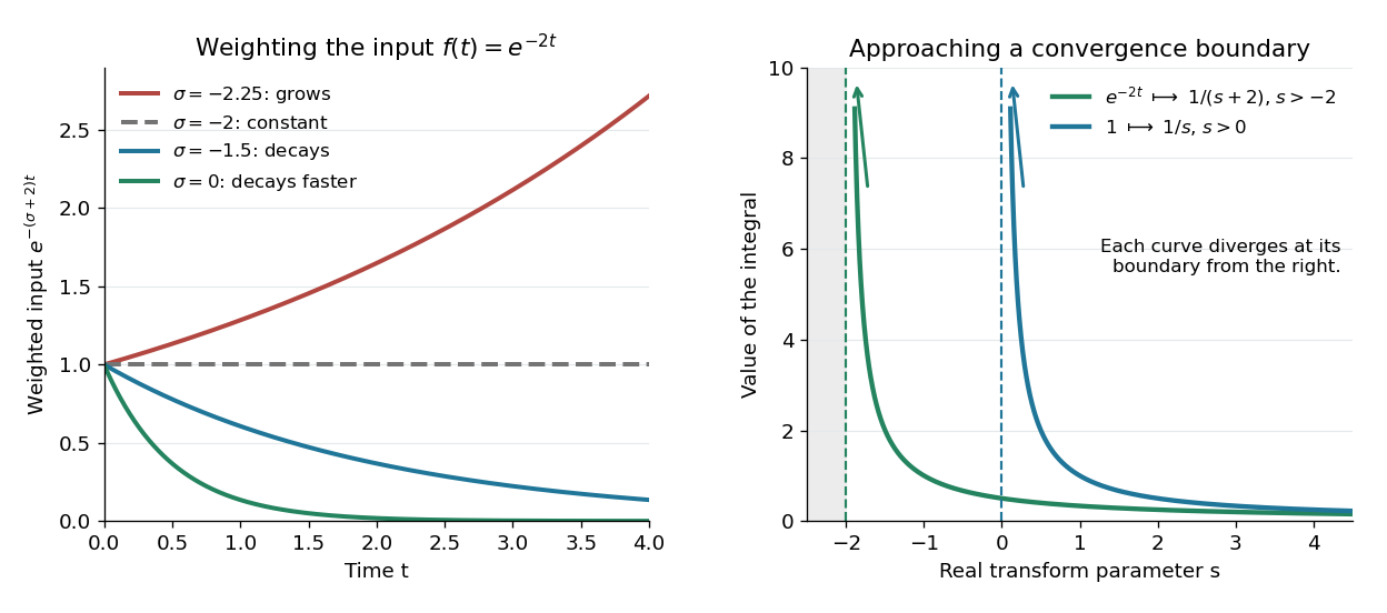
The bound has a short explanation. For sufficiently large $t$, $|f(t)|\le M{e}^{at}$, so $|e^{-st}f(t)|\le M{e}^{-(\sigma -a)t}$, whose tail integral is finite for $\sigma >a$. The finite initial interval is covered by piecewise continuity.

Three calculations make the convergence condition concrete. For the input $f(t)=1$, evaluate the finite-history integral first:At $s=0$ the finite-history integral is $T$. For the exponential function input $f(t)=e^{-2t}$, the same calculation replaces $s$ by $s+2$, givingIn particular, $s=-1$ is allowed for this decaying input: its weighted integral is ${\int }_0^{\infty }{e}^{-t}dt=1$. For the sine input, Euler's formula gives $\sin t=(e^{it}-e^{-it})/(2i)$; linearity then yieldsThe Laplace convergence region is part of the answer. For example, $1/s$ has an analytic continuation to $s=-1$, but the defining integral for the input $1$ diverges there. The sine calculation is also developed in MIT 18.03SC, further elementary transforms.

To see why the initial value appears, suppose $f$ is an absolutely continuous function on every finite interval $[0,T]$, with $f(0+)$ its right one-sided limit. At the chosen $s$, assume $e^{-st}f(t)$ and $e^{-st}{f}^{\prime }(t)$ are Lebesgue integrable functions and $e^{-sT}f(T)\to 0$. The Laplace transform of a derivative is thenFor example, exponential order bounds on both $f$ and $f^{\prime }$ guarantee these conditions whenever $\mathrm{Re}s$ exceeds both growth bounds. The initial value is the lower-end boundary contribution of integration by parts.

Consider the initial value problemWrite $Y=\mathcal{L}\{y\}$. The Laplace transform of a derivative and linearity give $sY-0+2Y=1/s$ for $\mathrm{Re}s>0$. A partial fraction decomposition therefore givesWe recognize the two elementary Laplace transforms already computed. Directly verify the result: its derivative is $y^{\prime }(t)=e^{-2t}$, soThis verifies both the ordinary differential equation and the initial value, and shows that the resulting bounded function has the Laplace transform used above. The response rises from zero toward $1/2$: at that value the input $1$ balances the term $2y$. The general method is described in MIT 18.03SC, solving initial value problems.

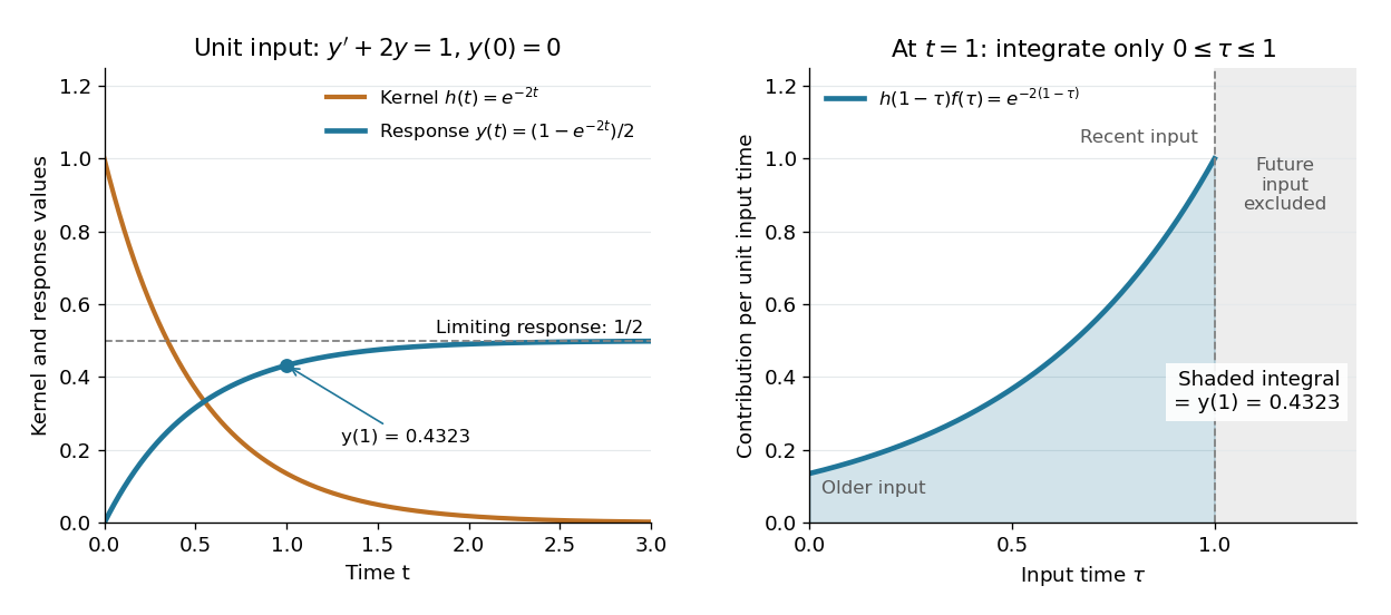
The same solution is a convolution. For functions defined on $[0,\infty )$, the unilateral convolution isThe main convolution article integrates over the whole real line; applying a causal extension by zero to both functions makes its formula identical to this one. Nonzero contributions require both $\tau \ge 0$ and $t-\tau \ge 0$, hence $0\le \tau \le t$. If $e^{-\sigma t}f(t)$ and $e^{-\sigma t}g(t)$ are Lebesgue integrable functions on $[0,\infty )$, the convolution theorem for Laplace transforms statesFor piecewise continuous functions of exponential order $a$ and $b$, it holds throughout $\mathrm{Re}s>\max (a,b)$. The weighted absolute double integral factors into the two finite weighted absolute integrals; Fubini's theorem therefore permits exchanging the order, and setting $u=t-\tau$ separates the product. ^[ref].

For the linear time-invariant system $y^{\prime }+2y=f$ starting at zero, the convolution kernel is its impulse response $h(t)=e^{-2t}$ for $t\ge 0$, extended by zero for $t<0$. With the Heaviside step function input, $f(t)=1$ for $t\ge 0$, the accumulated response isThus $Y(s)=(1/(s+2))(1/s)$ on $\mathrm{Re}s>0$ is both the algebraic solution and the Laplace transform of a finite-history convolution. Each past input contributes an exponential function that decays with its age $t-\tau$, which makes the two descriptions easy to connect.

Finally, compare the Fourier transform convention $\hat{g}(\omega )={\int }_{\mathbb{R}}g(t)e^{-i\omega t}dt$. If $f_0$ is the causal extension by zero of $f$, define $g_{\sigma }(t)=e^{-\sigma t}{f}_0(t)$. Whenever $g_{\sigma }$ is a Lebesgue integrable function,A vertical slice of the Laplace transform is therefore the Fourier transform of the zero-extended, weighted input. Positive $\sigma$ damps its positive-time history. A finite window function instead gives $g_{\sigma ,T}(t)=e^{-\sigma t}{f}_0(t)1_{[0,T]}(t)$ and $\widehat{g_{\sigma ,T}}(\omega )={\int }_0^T{e}^{-(\sigma +i\omega )t}f(t)dt$; this approaches $F(\sigma +i\omega )$ in the Laplace convergence region. Setting $\sigma =0$ directly requires an integrable zero-extended input: the input $1$ fails that condition, even though its Laplace transform exists for every $\sigma >0$.

The history of the Laplace transform spans several stages. Schiff's historical summary notes that Laplace's 1812 treatise acknowledged earlier work on integral transforms and describes later development of the modern Laplace transform method. ^[ref].

The Mellin transform is an integral transform suited to changes of scale: replacing $f(x)$ by $f(ax)$ multiplies its transform by $a^{-s}$ for $a>0$. For a locally integrable function $f:(0,\infty )\to \mathbb{C}$, definewhere the improper integral converges. The complex number $x^{s-1}=\exp ((s-1)\log x)$ uses the real natural logarithm because $x>0$. Its absolute value is $x^{\sigma -1}$, so absolute convergence depends on the real part $\sigma$ rather than the imaginary part $\tau$. The Mellin fundamental strip records the open range of such real parts.^[ref]

A familiar example is the exponential function $f(x)=e^{-x}$:This is exactly the Gamma integral. Near zero $e^{-x}$ tends to one, so absolute convergence requires $\sigma >0$; at infinity $x^r{e}^{-x}\to 0$ for every real $r$, so there is no upper boundary. The Gamma function has a meromorphic continuation with simple poles at $0,-1,-2,\dots$, but a finite continued value elsewhere in $\sigma \le 0$ does not make the defining improper integral converge.^[ref]

The Mellin transform of an interval indicator gives an elementary example with absolute convergence for every complex number $s$. The Mellin transform in logarithmic coordinates explains why changes of scale become translations, connecting the scaling property of the Mellin transform to the Fourier transform.

Use negative-exponential spatial Fourier transforms and finite-time spectral boundary transforms:Write $\mathcal{F}=k^2{F}_0-ik{F}_1-F_2$ and $\mathcal{G}=k^2{G}_0-ik{G}_1-G_2$. Integrate the local relation first over $0<x<L$ and then over time. The left and right endpoint fluxes have opposite signs, giving the finite-interval Airy global relationAll these spatial and temporal integral transforms are entire functions of $k$ for sufficiently smooth data on the finite intervals. Put $\alpha =e^{2\pi i/3}$ and $k_j={\alpha }^{j}k$, $j=0,1,2$. The dispersion relation obeys $\omega (k_j)=\omega (k)$; hence the same global relation holds at all three $k_j$. In particular, the missing traces satisfy the concrete linear systemwhere, with a common upper time limit $t$,The finite-time spectral boundary transforms $F_j,G_j$ are invariant under these rotations because their time kernel depends only on $k^3$. The coefficients multiplying them are not invariant; these differences make the three equations useful for eliminating the missing boundary traces.

Fix counterclockwise arclength on each side and take the outward normal derivative. WriteThe unit tangent is $i{c}_j$ and the outward unit normal is $c_j$. On side $j$ this gives the chain-rule identityPut $w=c_{j}k$. The exponential in the closed differential one-form pulls back toAlso $-\lambda qd\bar{z}/(ik)=(\lambda /w)q^{(j)}ds$. Consequently the contribution of side $j$ is ${\rho }_j(c_{j}k)$, where the required local side spectra areThese are spectral integral transforms in the local coordinate of each side. Keeping the tangential-derivative term is important: premature integration by parts in a single side integral would leave corner values, which cannot simply be discarded. At the special samples used below, those endpoint terms do vanish for the rotationally invariant solution.

Use the Bromwich inversion formula in the real variable $\omega$, with $p=\gamma +i\omega$:When the relevant Laplace transforms and spatial integral transforms are explicit, every sample of this integrand can be evaluated directly, without a time-stepping approximation to the partial differential equation. Split the initial condition integral at $y=x$: the two pieces of $R_q$ are linear combinations of $e^{\pm qy}$, so truncated spatial exponential transforms suffice. For real data the negative-frequency half is the complex conjugate of the positive-frequency half.

A practical numerical integration is to truncate to $|\omega |\le \Omega$, apply an adaptive quadrature rule, and independently increase $\Omega$ and refine the quadrature. Choose $\gamma >0$ large enough to remain to the right of all singularities, but avoid an unnecessarily large $e^{\gamma t}$. Evaluate hyperbolic function ratios in scaled form; for example,This prevents overflow when $\mathrm{Re}qL$ is large. The boundary contributions at an interior point are damped by $e^{-x\mathrm{Re}q}$ or $e^{-(L-x)\mathrm{Re}q}$, with $\mathrm{Re}q\sim \sqrt{|\omega |/2}$. Near an endpoint more frequencies are needed; at the endpoint itself use the prescribed Dirichlet boundary condition. The initial condition resolvent has a generally only $O(1/\omega )$ tail. Treat its oscillatory tail accurately, subtract a known transform with the same leading term, or evaluate that contribution separately with the heat kernel.

An equally useful check is the eigenfunction expansion. DefineThe causal modal formula isIt follows either from the heat kernel formula or directly from integration by parts against a sine eigenfunction. Exponential-transform formulas evaluate the time integral explicitly when available. The initial condition contribution has a Gaussian function cutoff in $n$ for each positive time. Nonzero endpoint forcing produces a more slowly convergent sine series tail. A boundary lifting $\ell (x,t)=(1-x/L)g_0(t)+(x/L)e^{aL}h(t)$ gives $w=\ell +z$, where $z$ has zero Dirichlet boundary conditions and forcing $-{\ell }_t-a^2\ell$; expanding $z$ gives better convergence and imposes the endpoint values exactly. At very small times the method of images is often more efficient than retaining many modes.

Check convergence by increasing both the frequency cutoff and quadrature resolution, and compare with a separately truncated causal modal or image-kernel evaluation. Causality in finite-time Laplace contour inversion means a leftward contour deformation must respect both resolvent operator poles and growth of the transformed data. In particular, the transform of data extended by zero after $T$ can grow like $e^{-pT}$ in the left half-plane: for $t<T$ one cannot close that contour indiscriminately and discard its large arc. The modal forcing integral with upper limit $t$ avoids this causality error.

Put $a=\alpha /2$ and apply the Dirichlet gauge transform for constant drift $w(x,t)=e^{ax}u(x,t)$. Taking derivatives directly removes the advection term and gives the damped heat equation $w_t=w_{xx}-a^{2}w$. Thus $w_0(y)=e^{ay}{u}_0(y)$, while the two Dirichlet boundary conditions become $w(0,t)=g_0(t)$ and $w(L,t)=e^{aL}h(t)$.

The Dirichlet heat kernel on an interval and its damped version areThe method of images gives an alternative, often better at short times:To determine the boundary signs, multiply the equation for $w$ by the backward heat kernel $K_a(x,y,t-s)$ and use integration by parts in $y$. Since the kernel vanishes at $y=0,L$, the surviving boundary expression is $K_{a,y}(x,0,t-s)g_0(s)-K_{a,y}(x,L,t-s)e^{aL}h(s)$. Consequently an integral representation containing only the given data isThis is a Dirichlet boundary-forcing heat-kernel formula. For $0<x<L$ the short-time Gaussian decay makes the forcing integral well defined. The endpoint values are interior limits of the complete formula: evaluating a termwise sine series at an endpoint before taking the time integral loses the nonzero boundary values. At the initial corners a continuous classical solution requires $u_0(0)=g_0(0)$ and $u_0(L)=h(0)$; otherwise the same formula describes the solution away from those corners.

Here is a second integral representation, useful when the integral transforms are explicit. Extend $g_0,h$ by zero after $T$; the values of the extension cannot affect a solution at $t<T$. Write their Laplace transforms as $G(p),H(p)$ and set $q=\sqrt{p+a^2}$ using the principal square root. The transformed Dirichlet Green function for $-{\partial }_x^2+q^2$ isIt vanishes at both endpoints and its first derivative in $x$ jumps by $-1$, which verifies the sign of its unit source. The resolvent kernel for Dirichlet advection-diffusion on an interval gives the transformed solutionThe Bromwich inversion formula therefore yieldsThe square-root notation creates no genuine branch singularity here: all three kernels are even in $q$. Their only spatial resolvent operator poles are $p=-a^2-q_n^2$. This transformed formula and the causal heat kernel formula represent the same solution in the usual smooth-data class.