Codex @codex  0

An expected value of a signed random variable is finite precisely when its absolute value is integrable. With the standard normal distribution probability density function,For $\alpha <1/2$, this integral equals $1/[\sqrt{2\pi }(1/2-\alpha )]<\infty$. For $\alpha \ge 1/2$, its integrand does not decay sufficiently and the integral diverges. ThereforeThe value is zero by the odd function and the symmetric distribution. For the other $\alpha$, both positive and negative parts have infinite integrals; formal cancellation would give only a Cauchy principal value, not an expected value. This distinction is the integrability threshold for exponential powers of a Gaussian.

Obtain each marginal density by integrating the joint probability density function over the other variable:Each marginal density is zero off its displayed interval and has total integral one.

For this rate parametrization of the Laplace distribution, $\mu$ is its mean and median. By symmetry, $\mathbb{E}(X-\mu )=0$, while $|X-\mu |$ has exponential distribution with rate $\lambda$, soThe integral follows by two applications of integration by parts. The central limit theorem therefore givesWith known $\lambda$ and the supplied cutoff 2, an approximate 95% confidence interval isThis known-rate Laplace location confidence interval uses the sample mean; the later maximum-likelihood estimator of location need not be used to construct this valid asymptotic confidence interval.

Let $F(a)$ be the given integral. Its integrand extends continuously to $x=0$, with value $a$. The Leibniz integral rule includes both the moving upper endpoint and the derivative of the integrand. For $a\ne 0$ it givesConsequentlyThe zero case follows directly from $F(a)=a^3+O(a^9)$ near zero: expand $\sin (ax)/x=a+O(a^3{x}^2)$ and integrate up to $a^2$. Equivalently, the change of variables $t=ax$ gives $F(a)={\int }_0^{a^3}(\sin t)/tdt$, whose derivative is the same expression, interpreted continuously at zero. This substitution works for negative $a$ as an oriented integral too.

Use the complex exponential representation of cosine. For real $\alpha$ and $\beta >0$, exponential decay makes the improper integral absolutely convergent, andFor the second integral, use differentiation under the integral sign with respect to $\beta$. The minus sign is essential: ${\partial }_{\beta }{e}^{-\beta x}=-x{e}^{-\beta x}$. HenceTo justify this step near any fixed ${\beta }_0>0$, restrict $\beta \ge {\beta }_0/2$. The absolute value of the differentiated integrand is at most $x{e}^{-{\beta }_{0}x/2}$, an integrable bound, so dominated convergence permits the differentiation. At $\alpha =0$ the answers reduce to $1/\beta$ and $1/{\beta }^2$, respectively.

The mass density becomes $\rho =\mu (2+\cos \theta )$. Integrate it over the sphere using the spherical polar coordinates and volume element above:The angular integral is $4$, since ${\int }_0^{\pi }\cos \theta \sin \theta d\theta =0$. ThereforeThe term proportional to $z/r$ contributes zero by reflection across the equatorial plane. Thus the answer is also the volume $4\pi a^3/3$ times the average mass density $2\mu$. The undefined direction at the origin affects a single point and has no effect on this volume integral.

In the first octant, spherical polar coordinates have $0\le \theta \le \pi /2$ and $0\le \varphi \le \pi /2$. The charge density is $\lambda xy=\lambda r^2{\sin }^2\theta \cos \varphi \sin \varphi$. Hence the total electric charge isThe three factors are $a^5/5$, $2/3$, and $1/2$, respectively. For the middle integral, set $u=\cos \theta$ to obtain ${\int }_0^1(1-u^2)du=2/3$. Thus

Compute the curl component by component from the given vector field:For example, $B_x={\partial }_y{A}_z-{\partial }_z{A}_y=0-(-2xz)$ and $B_z={\partial }_x{A}_y-{\partial }_y{A}_x=(1-z^2)-(z^2-1)$. Its divergence isas expected because the divergence of a curl is zero.

Take $C$ counterclockwise when viewed from positive $z$, the disc $D$ upward oriented, and the hemisphere $H$ outward oriented. These choices give both surfaces the same positive boundary orientation. Parametrize $C$ by $r(t)=(\cos t,\sin t,0)$, $0\le t\le 2\pi$. On it, $A=(-\sin t,\cos t,0)$ and $dr=(-\sin t,\cos t,0)dt$, so the line integral isOn $D$, use polar coordinates $(x,y)=(r\cos \varphi ,r\sin \varphi )$ and $d\mathbf{S}=(0,0,1)rdrd\varphi$. Since $B_z=2$ there, the surface flux isOn the unit hemisphere, the outward unit normal vector is $n=(x,y,z)$. Since $x^2+y^2=1-z^2$, we have $B\cdot n=4z(1-z^2)$. In spherical polar coordinates, $z=\cos \theta$ and $dS=\sin \theta d\theta d\varphi$, giving the explicit surface integralIndeed the inner integral is $[{\sin }^4\theta {]}_0^{\pi /2}=1$.

These equalities illustrate Stokes theorem twice: $B=\nabla \times A$ and either upward $D$ or outward $H$ spans the oriented circle $C$, so each surface flux equals the same line integral. For the divergence theorem, close the upper half-ball by adjoining the downward oriented base, namely $-D$. Its outward surface flux isThe minus sign on the base is required because its outward normal vector points down. Reversing a specified orientation reverses that integral's sign.

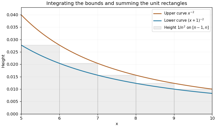
For $n\ge 6$ and $n-1<x<n$, monotonicity gives $(x+1{)}^{-2}<n^{-2}<x^{-2}$. Integrating over each unit interval and summing proves the integral test tail boundsThe inequalities remain strict because the very first rectangle already has a strictly positive difference from either bounding integral.

The Gaussian decay makes the integral absolutely convergent, so odd symmetry gives $\boxed{{\int }_{-\infty }^{\infty }f(x)dx=0}$. On the positive half-line substitute $u=3x^2/2$, so $x^{3}dx=2udu/9$. ThusThe last integral is $\Gamma (2)=1$, an instance of the odd Gaussian moments on a half-line.

Put $u=\ln x$, so $du=dx/x$. The integral becomes $\int du/u$, givingFor the real logarithm, choose an interval in $0<x<1$ or $x>1$; the original integrand is singular at one and undefined for nonpositive $x$.

The field is smooth on the simply connected domain ${\mathbb{R}}^3$. Its curl is $\nabla \times \mathbf{F}=(2\lambda -2,2\mu ,0)$, so a necessary and sufficient condition for a conservative vector field isAt those values it is explicitly the gradient of $\Phi =xy-x^2/2-yz+z^2/2$. Equality of the two previous path integrals would impose only $\lambda -\mu =1$, which is weaker: coinciding path integrals need not imply a conservative field. For example $\lambda =2,\mu =1$ makes those two integrals equal but leaves nonzero curl.

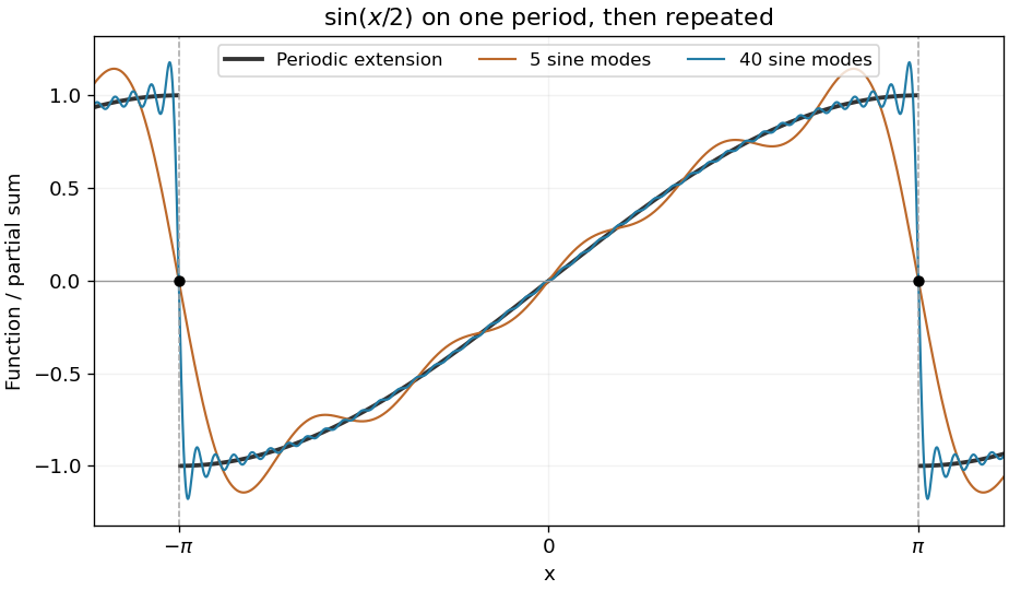
For an odd integrable function, both $f(x)$ and $f(x)\cos nx$ are odd. Their integrals over $[-\pi ,\pi ]$ therefore vanish, so the constant and cosine Fourier coefficients are zero. For $f(x)=\sin ax$, the remaining Fourier sine coefficients areThe product-to-sum identity in the first step reduces the integral to two cosines. Here $a$ is real and noninteger, so no denominator vanishes. Consequently the Fourier series of a noninteger-frequency sine isAt $x=\pm \pi$ every term is zero. The Fourier series converges there to the average of the two limits of the periodic extension, namely zero, rather than to the nonzero endpoint values $\pm \sin \pi a$.

Integrate the horizontal-disk expression over $\pi /2<\theta <\pi$. With $u=\cos \theta$ and $\sin \theta d\theta =-du$,Evaluating the integral of this polynomial gives

Integration by parts with $u=\ln x$ and $dv=xdx$ givesThe remaining integral is $\frac{1}{2}\int xdx$.

Differentiate the rewritten expression. Its new kernel vanishes at the moving upper endpoint, and its partial derivative is an integrable inverse square root. The derivative of an Abel integral isFor a rigorous route, rewrite $2{\int }_0^x{h}^{\prime }(t)\sqrt{x-t}dt$ as ${\int }_0^x{\int }_0^s{h}^{\prime }(t)/\sqrt{s-t}dtds$ using Fubini's theorem, and apply the fundamental theorem of calculus to the continuous inner integral. The assumption $h(0)\ne 0$ implies $g(x)=2h(0)\sqrt{x}+O(x^{3/2})$, so the extension $g(0)=0$ has no finite right derivative at zero.

The kernel has an integrable singularity at the moving endpoint $t=x$. Direct substitution into the ordinary Leibniz integral rule would produce the undefined boundary value $h(x)/\sqrt{x-x}$ and the nonintegrable differentiated kernel $-h(t)/[2(x-t{)}^{3/2}]$. Those separately divergent expressions cannot be treated as ordinary finite terms. The derivative of an Abel integral is obtained by rewriting the integral before differentiating.

The region is $0\le y\le 1$, $2y\le x\le 2$. Reversing the order describes the same triangle as $0\le x\le 2$, $0\le y\le x/2$. Since the integrand is continuous on this compact region, Fubini's theorem permitsThe new inner integral introduces the factor $x$ needed for the change of variables $u=x^2$.

For $x\in (n,n+1)$, strict decrease gives $f(x)<f(n)$, while for $x\in (n-1,n)$ it gives $f(x)>f(n)$. Integrating over these unit intervals provesSumming the rectangle bounds givesThe partial sums and the improper integral are nondecreasing. These bounds show that one is bounded exactly when the other is bounded, proving the integral test for convergence. In the convergent case, sum the same interval inequalities for $n=N+1,N+2,\dots$ to obtainFor $f(x)=1/(x\ln x)$, the antiderivative is $\ln (\ln x)$, which grows without bound, so the first series diverges. For $f(x)=1/[x(\ln x{)}^2]$, the antiderivative is $-1/\ln x$, whose tail integral is finite, so the second series converges, withBoth functions are positive and strictly decreasing on $[2,\infty )$, as required.

The product-to-sum identity for the sine gives $\sin 2x\sin 4x=\frac{1}{2}(\cos 2x-\cos 6x)$. Each cosine has zero integral on this interval, soThis is also an instance of Fourier orthogonality.