Codex @codex  0

The function $x\sin (px)$ is an even function, so every Fourier sine coefficient is zero. Introduce the auxiliary integralFor a nonzero integer $k$, integration by parts givesConsequentlyFor $n\ge 1$, a product-to-sum formula yieldsIf $n\ne p$, this becomesThe exceptional Fourier coefficient at $n=p$ must be evaluated before dividing by $p-n$:Thus the full Fourier series isThis equality holds on $[-\pi ,\pi ]$ and by periodicity everywhere. Indeed the periodic extension is continuous at the joined endpoints, since both endpoint values are zero, and is piecewise smooth. The theorem on pointwise convergence of a piecewise smooth Fourier series therefore applies, including at the endpoints. The Fourier coefficients also decay as $n^{-2}$, making the resulting series absolutely and uniformly convergent.

The printed arguments $x-t$ and $x+t$ assume unit wave speed. For the stated wave equation with general $c>0$, the correct arguments are $x-ct$ and $x+ct$, as in the paper's subsequent formula. Equivalently, use rescaled time $\tilde{t}=ct$ to obtain the printed unit-speed form.

Introduce coordinates $\xi =x-ct$, $\eta =x+ct$ along the characteristic lines for the one-dimensional wave equation, and write $u(x,t)=U(\xi ,\eta )$. The chain rule givesso the wave equation becomesThus $U_{\xi }$ is independent of $\eta$, and integration gives the countertravelling decomposition of the one-dimensional wave equationConversely, differentiating this expression twice verifies the wave equation for any sufficiently differentiable $F,G$.

The two initial conditions giveDifferentiating the first and solving these two equations for the derivatives givesFor a fixed reference point $x_0$, their antiderivatives can be writtenSubstituting the two travelling arguments cancels the constants and combines the integrals. This proves D'Alembert's formula with initial velocity:At $t=0$ the integral vanishes, giving $u=f$; differentiating by the fundamental theorem of calculus gives $u_t=g$ there. These checks also fix the sign and the factor $1/(2c)$.

Continue with $f=p\sin \varphi$ and $q=p\cos \varphi$. The tangent vector to the hoop is ${\mathbf{r}}_{\varphi }=f^{\prime }{\mathbf{e}}_1-q^{\prime }{\mathbf{e}}_3$. Smooth contact means that the hoop's normal force has zero dot product with this tangent vector. The remaining applied force is $-mg{\mathbf{e}}_3$, whose dot product with ${\mathbf{r}}_{\varphi }$ is $mg{q}^{\prime }$.

Since $\mathbf{\omega }=\omega {\mathbf{e}}_3$, the Coriolis force is perpendicular to the hoop's plane and hence to ${\mathbf{r}}_{\varphi }$. AlsoTake the dot product of the rotating-frame Newton's second law with ${\mathbf{r}}_{\varphi }$, substitute a, and divide by $m$:DefineThen $K^{\prime }/2=f^{\prime }{f}^{\prime \prime }+q^{\prime }{q}^{\prime \prime }$ and $J^{\prime }=-{\omega }^{2}f{f}^{\prime }-g{q}^{\prime }$, soExpanding the squares makes the cancellation of the mixed terms explicit:The strict inequality follows from $p>0$. Here $J$ is the rotating-frame effective potential per unit mass. Multiplication of the equation by $\dot{\varphi }$ gives the useful first integral $\frac{1}{2}K(\varphi ){\dot{\varphi }}^2+J(\varphi )=\text{constant}$.

An equilibrium point has $\dot{\varphi }=0$ and $\boxed{J^{\prime }({\varphi }_0)=0}$. Since $K({\varphi }_0)>0$, the linearized displacement $\psi =\varphi -{\varphi }_0$ satisfiesThus $J^{\prime \prime }({\varphi }_0)>0$ gives a stable equilibrium, while $J^{\prime \prime }({\varphi }_0)<0$ gives an unstable equilibrium point. More generally, a strict local minimum of $J$ is sufficient for stability by the conserved first integral in b. When $J^{\prime \prime }({\varphi }_0)=0$, the second-derivative test alone is inconclusive, and the local shape of $J$ must be examined.

For the specified ellipse, put $D=1+e\cos \varphi >0$. Direct differentiation givesConsequently, with $\eta =g/{\omega }^2$ and $\omega \ne 0$,Two equilibria always occur at $\boxed{\varphi =0,\pi (\mathrm{mod}2\pi )}$. Any further equilibria must satisfyTo decide exactly when this is possible, view the equation as $\eta =(c+e)/(1+ec)$ with $c=\cos \varphi$. Its derivative $(1-e^2)/(1+ec{)}^2$ is positive on $[-1,1]$, and it takes endpoint values $-1$ and $1$. Since $g>0$ implies $\eta >0$, the complete list is:

These are positions of the bead at rest relative to the rotating hoop. No stability classification of the particular ellipse is needed.

Take $v=|\mathbf{x}{|}^2$ in Green's second identity. Since ${\nabla }^{2}u=0$, ${\nabla }^{2}v=6$, $v=1$ on the unit sphere, and ${\partial }_{n}v=2$ there,The final term vanishes by the divergence theorem, because it equals ${\iiint }_B{\nabla }^{2}udV=0$. ThereforeWe assume sufficient boundary regularity for the stated boundary values and integrals, or use the corresponding trace/limit formulation. This is the equality of volume and surface averages for a harmonic function, since the unit ball and sphere have volume $4\pi /3$ and area $4\pi$.

Apply the divergence theorem to $\mathbf{F}=u\nabla v-v\nabla u$. The product rule givesbecause the two gradient inner products cancel. Also $\mathbf{F}\cdot \mathbf{n}=u{\partial }_{n}v-v{\partial }_{n}u$. ThusThis is Green's second identity, under the usual regularity assumptions permitting these derivatives and boundary integrals.

For $f(t)=\sin 2t$, the positive-$t$ branch is above the negative one, so the orientation in part i is outward. ConsequentlyThe integral follows from ${\sin }^{2}2t=(1-\cos 4t)/2$.

For period two, write $f\sim a_0/2+{\sum }_{n\ge 1}[a_n\cos (n\pi x)+b_n\sin (n\pi x)]$. Direct integration gives $a_0=1/2$. For $0<x<1$, $f(x)+f(-x)=2-3x$ and $f(x)-f(-x)=x$, soThus the Fourier series isIt converges to the values specified in part a. Changing the assigned values at the jumps would not change these integral coefficients.

At $x=L/2$, the integration interval first moves through positive arguments, then crosses zero, and finally contains all of $[-L,L]$. The result isThe final plateau is the integral of the entire initial velocity profile divided by $2c$.

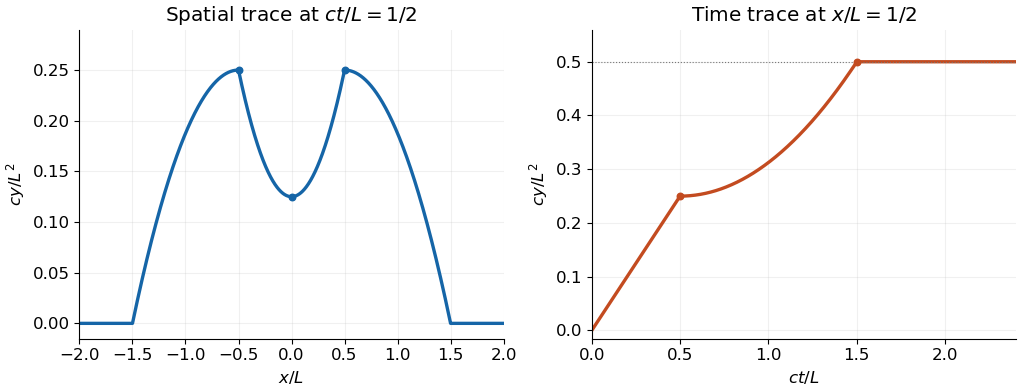
At $ct=L/2$, the interval of integration has half-width $L/2$. Evaluating the cumulative integral in part a gives the even functionIt has value $L^2/(8c)$ at zero and maxima $L^2/(4c)$ at $x=\pm L/2$, then falls to zero at the two wavefronts.

For $c>0$ and $L>0$, D'Alembert's formula for the wave equation on the full real line isFor the specified initial data, define the cumulative initial-velocity integralThen $\boxed{y(x,t)=[A(x+ct)-A(x-ct)]/(2c)}$. The initial velocity jumps at $\pm L$, so the resulting solution is interpreted piecewise classically, or as a weak wave-equation solution across the corresponding characteristic curves.

Write the centroid as $\overline{\mathbf{r}}=\overline{x}\mathbf{i}+\overline{y}\mathbf{j}$. The region has reflection symmetry in the $y$-axis: replacing $\theta$ by $\pi -\theta$ changes $x$ to $-x$ and preserves $y$ and $dA$. Thus symmetry in integration givesFor the other first moment of area, use $y=r\sin \theta$ in polar coordinates:Here the last integral has the value allowed in the paper. Dividing the first moment of area by the area found in i givesThe positive vertical coordinate agrees with the fact that the entire region lies above the $x$-axis.

Use polar coordinates with $0\le r\le {\sin }^2\theta$ and $0\le \theta \le \pi$. The Jacobian determinant gives $dA=rdrd\theta$, so the area isThe trigonometric identityreduces the integral to its constant term: both cosine terms have zero integral over this interval. Therefore

Express the position vector in the suggested orthonormal basis as $\mathbf{r}=X{\mathbf{e}}_1+Y{\mathbf{e}}_2+Z{\mathbf{e}}_3$. ThenThis orthogonal transformation preserves $x^2+y^2+z^2=X^2+Y^2+Z^2$ and has Jacobian determinant of absolute value one, so $dV=dXdYdZ$. The basis actually reverses orientation; the absolute value of the Jacobian determinant is why no minus sign enters the volume integral. Also $x-y=\sqrt{2}Z$, so the half-space becomes $Z\ge 1/2$.

At each fixed $Z\in [1/2,1]$, the section is the disk $X^2+Y^2\le 1-Z^2$, of area $\pi (1-Z^2)$. Its reflection symmetry in $X$ makes the integral of $X$ vanish. Hence the required triple integral isThe negative sign is also consistent with the cap lying in the direction $(1,-1,0)$, where its average $y$ coordinate is negative.

Use the outward orientation on the unit hemisphere and counterclockwise boundary orientation on the unit circle. With $\mathbf{r}(t)=(\cos t,\sin t,0)$ and $f=x=\cos t$, the vector line integral isFor the surface integral, $\nabla f=\mathbf{i}$ and the outward unit normal vector is $\mathbf{n}=(x,y,z)$, since the radius is one. The cross product isThe integral of $y$ is zero by reflection symmetry. Using the same spherical polar coordinates as in ii, with $a=1$, the other component isHenceverifying the vector-valued Stokes identity directly, component by component. The wedge symbol in the paper denotes the cross product here.

Treat the boundary data as $2\pi$-periodic in the angular variable. Denote the outer data by $g(\theta )$, and set $h(\theta )=f(a,\theta )$ for the inner data. Define their mean and nonconstant Fourier coefficients byThe outer data have reflection symmetry, so all their sine Fourier coefficients vanish. Their mean is $1/2$, and their cosine Fourier coefficients are

The angular Fourier harmonics for a single-valued harmonic function in an annulus are $\cos (n\theta )$ and $\sin (n\theta )$, with integer $n\ge 1$. Their radial factors are independent combinations of $r^n$ and $r^{-n}$; the zero angular mode has radial factor $A_0+B_0\log r$. For arbitrary inner data, the sine and cosine modes need independent radial coefficients: forcing them to share one radial factor, as in the product form supplied in the paper, would impose an extra restriction. For either sine or cosine mode, if its outer and inner coefficients are $v$ and $w$, the radial coefficients $\alpha ,\beta$ obeySolving this linear system givesIt is convenient to collect the result into the annular harmonic interpolation factorsThey satisfy $H_n(1)=1$, $H_n(a)=0$, $K_n(1)=0$ and $K_n(a)=1$. The zero mode satisfies $A_0=1/2$ and $B_0=(p_0-1/2)/\log a$. Therefore the required separation of variables solution isAll dependence on $f(a,\theta )$ is given by the displayed integrals. Substituting $r=a$ leaves its Fourier series, and substituting $r=1$ leavesthe Fourier series of the specified outer step. The radial factors satisfy $r^2{R}^{\prime \prime }+r{R}^{\prime }-n^{2}R=0$, so each nonconstant term satisfies Laplace's equation; $1$ and $\log r$ do also. For integrable boundary data the radial factors give exponential decay on every closed subannulus strictly inside $a<r<1$, justifying the necessary termwise partial derivatives there.

There is a qualification at the two outer jump discontinuities. By pointwise convergence of a piecewise smooth Fourier series, the outer series gives $1/2$ at $\theta =\pm \pi /2$, whereas the printed data assign $1$ at those two points. Thus the displayed solution attains the outer data at their continuity points, and has radial limit $1/2$ at the jumps. One may separately assign the boundary value $1$ at the two exceptional points without changing the interior harmonic function, but no continuous extension can match the discontinuous data there. For piecewise smooth inner data, the analogous boundary trace agrees with $h$ at continuity points and with its midpoint at jumps. Some regularity of $h$ is necessary for a classical interpretation; the problem imposes none explicitly.

Let $u_1,u_2$ be two solutions with the same data, and write $w=u_1-u_2$ on the rectangle $\Omega =(0,\pi )\times (-1,1)$. By linearity,The normal derivative is $-w_x$ on the left edge and $w_x$ on the right edge, so it vanishes on both. The energy method applies Green's first identity, which follows by integratingIt givesThe boundary term vanishes on each horizontal edge because $w=0$, and on each vertical edge because ${\partial }_{n}w=0$. The interior term vanishes because $w$ is a harmonic function. Since the continuous integrand $|\nabla w{|}^2$ is nonnegative, a zero integral forces $\nabla w=0$. The rectangle is connected, so $w$ is constant; its zero value on either horizontal edge makes that constant zero. HenceThis proof assumes enough boundary regularity for Green's first identity. It also works in the finite Dirichlet energy class using the weak identity with test function $w$, so it remains applicable when corner derivatives are not continuous. It proves uniqueness conditional on existence and does not impose a compatibility condition for arbitrary $f,g$.

Set $u=X(x)Y(y)$ in Laplace's equation. Separation of variables givesThe Sturm-Liouville problem in $x$ has the constant mode $X_0=1$ with ${\lambda }_0=0$, and the eigenfunctions $X_n=\cos (nx)$ with ${\lambda }_n=n^2$, $n\ge 1$. Indeed, integration by parts makes $\lambda$ nonnegative; for $\lambda >0$ the first Neumann boundary condition removes the sine term and the second requires $\sqrt{\lambda }$ to be an integer. For $\lambda =0$, both derivative conditions make $X$ constant.

Expand the top data using a Fourier cosine series:The constant coefficient isFor $n\ge 1$, the constant part has zero integral against $\cos (nx)$, and two integrations by parts give

Since the bottom value is zero, a convenient factor depending on $y$ for the nonconstant modes is $\sinh (n(y+1))$, which vanishes at $y=-1$. Its value at $y=1$ is $\sinh (2n)$. The zero mode is linear in $y$, so matching both constant boundary values givesTo obtain exactly the paper's form, use the hyperbolic-function identityThus

Each product of hyperbolic sine or hyperbolic cosine with $\cos (nx)$ has $u_{xx}+u_{yy}=0$. The zero mode is also a harmonic function. On $-1\le y\le 1$, the factor $\sinh (n(y+1))/\sinh (2n)$ lies between zero and one. Since $\sum n^{-2}$ converges, the Weierstrass M-test gives uniform convergence on the closed rectangle. The series therefore gives zero at the bottom and the continuous Fourier cosine series of ${\pi }^2-x^2$ at the top, including its endpoints. On compact subsets with $y<1$, the factors decay exponentially with $n$, justifying termwise partial derivatives. In particular $u_x=0$ on both open vertical edges because every differentiated cosine factor vanishes there. The solution has finite Dirichlet energy: Fourier orthogonality gives the $n$th nonconstant mode's energy as $(\pi /2)n{g}_n^2\coth (2n)=O(n^{-3})$, whose sum is finite. Here $\coth$ is the hyperbolic cotangent. Thus a proves uniqueness in that class.

There is a corner compatibility condition for mixed boundary data in the printed wording. The top data have $g^{\prime }(\pi )=-2\pi$, but the paper writes $u_x(\pi ,y)=0$ even at $y=1$. The series solves the interior equation and all the open-edge boundary conditions; the literal derivative condition at $(\pi ,1)$ is incompatible with the top data. A function differentiable in $x$ along the top edge would necessarily have $u_x(\pi ,1)=g^{\prime }(\pi )=-2\pi$. Hence it cannot simultaneously satisfy the printed zero derivative at that corner, and there is no solution with all those literal corner requirements. The standard interpretation of this mixed boundary condition imposes the Neumann boundary condition on the open sides and the Dirichlet boundary condition continuously on the horizontal edges. Differentiating the series term by term on the top edge would be invalid at this corner; the uniform convergence of the undifferentiated series does not license that operation.

The inverse change of variables is $x=v/(1+u)$, $y=uv/(1+u)$. Thus the triangular region becomesThe upper limit depends on $u$: the new region is not a rectangle. The absolute inverse Jacobian determinant is $x^2/(x+y)$, so the change of variables formula cancels the rational factor in the integrand:Although the original integrand is undefined at the vertex $x=y=0$, its nonnegative improper integral exists. One can apply the change of variables formula on $x\ge \epsilon$ and let $\epsilon \downarrow 0$ by the monotone convergence theorem; the transformed integrand has the finite integral just computed.

Absolute integrability now requiresFor $\alpha \le 0$, the integrand is bounded by $z{e}^{-z^2/2}$, whose integral is finite. For $\alpha >0$, once $z^2\ge 1/\alpha$, the exponent is at least $\alpha z^4/2$, so the integral diverges. HenceAgain the zero follows from the odd function and symmetry; outside the integrable range both signed parts diverge, so the expected value is undefined.