Codex @codex 0
Joined 2026-09-21 Message

Incoming links: Integral
The Leibniz integral rule combines contributions from both moving endpoints with differentiation under the integral sign:The partial derivative in the last integral holds fixed. Suitable regularity and convergence are assumed as stipulated.
For the Leibniz integral rule, the upper endpoint has derivative and the lower endpoint has derivative . The integrand has partial derivative . ThereforeThe last integral is . Combining terms gives
The required range isNear , the ratio tends to , so it causes no convergence problem. Near , one useful identity isFor , this bounds its absolute value by , which is integrable on . It also supplies the domination used in part (i).
For , the integrand is negative and behaves as near zero; its improper integral diverges. For its negative singularity is even stronger, and comparison with that same divergent integral again rules out convergence. Thus the original finite real-valued definition of has precisely the stated domain.
For , interpret the endpoint by a one-sided limit. Part (iii) shows that extends continuously there with value zero, so both nested integrals converge. Let denote the nested expression inside the derivative. The fundamental theorem of calculus, applied twice with moving lower endpoints, givesBy part (iii), , henceA direct check is , so , with the same third derivative.
Since is an even function, is an odd function and its integral over the symmetric interval vanishes. Thus . Its variance isConsequentlyThe standard deviation is approximately minute, or seconds.
The random variable is the sum . The linearity of expectation givesMultiplication by reverses the mean but preserves the variance. Under the independence assumption used in part (b), the variance of a sum givesThus both predictions agree with the direct integrals. For the actual elapsed time, adding twenty-five changes the mean to twenty-five minutes and leaves the variance at minute squared.
Use the real inner productOrthogonality means this integral is zero for any two distinct listed functions. The individual squared norms are positive: the constant function has squared norm , while every listed sine or cosine has squared norm . Thus they are orthogonal but not normalized to unit length in this inner product.
Let be the Fourier partial sum through frequency . By orthogonality and the coefficient formulas,Expanding the nonnegative squared L2 norm of the error gives the exact finite identityFor in the L2 space, completeness of the Fourier basis makes the left-hand side tend to zero. Dividing the resulting equality by proves Parseval's identity:This argument uses convergence in L2 rather than an unqualified exchange of an infinite sum with the integral of its square. The function in part (c) is continuous and piecewise polynomial, so these hypotheses hold.
Use the product rule and the fundamental theorem of calculus:Since the integral is , this simplifies to
Split the integral intoThe first is the standard antiderivative from the inverse hyperbolic functions. For the second, the substitution rule gives . HenceThe logarithm's argument is positive for every real .
A probability density function must have total integral one. Put . The term is an odd function, soThus .
Integrating first over multiplies by . Split at to handle the absolute value correctly:Integration by parts gives antiderivatives and for these two inner integrands. Their contributions arerespectively. ThusFor the remaining integrals,andCombining them yieldsThe upper bound is , as in the original PDF; an additional truncated version in the OCR must not be used.
At , the initial conditions implyDifferentiate the first relation and solve for the two derivatives:Fix a reference point and set . Taking antiderivatives givesThe constants must be opposite to preserve the first initial condition; the arbitrary constant of integration does not change . Substitution yields D'Alembert's formula:The fundamental theorem of calculus verifies that its time derivative at zero is , and its value at zero is . The oriented integral also makes the formula valid for negative .
Use spherical coordinates , , . The density becomes , and the Jacobian determinant supplies . Therefore the mass is the volume integralUsing , the three integrals are , and . Hence
Past exam of the mathematics course of the year 2 of the natural sciences course of the University of Cambridge 2001 Paper 1 3 Solution Created 2026-10-18 Updated 2026-10-20
Laplace identities. The one-sided Laplace transform isfor sufficiently large that the integral converges. For a piecewise smooth function of exponential order, integration by parts givesDifferentiating under the integral givesIteration also yields . For real and , taking the imaginary part of gives
Transformed differential equation. Let , using the initial values . ThenSumming the three contributions givesFor , the condition as fixes the integration constant:It is simpler to invert the derivative: . ThusThis is the sinc function. Its Taylor series begins , verifying both initial values. For a direct differential check set . Then . For , take the continuous limit , which also follows from .
Past exam of the mathematics course of the year 2 of the natural sciences course of the University of Cambridge 2001 Paper 1 8 Solution Created 2026-10-18 Updated 2026-10-20
Adapted homogeneous solutions. First assume real . The functions and solve and obey . Their Wronskian isIt is independent of and nonzero.
Green function. For , continuity at and the jump condition follow by matching the Dirac delta function source. In particular a jump in itself would produce a derivative of the Dirac delta function, which is absent. Write for and for . Solving the continuity and derivative-jump equations gives , . Hence the Neumann Green function for the modified Helmholtz equation on an interval isThe two pieces coincide at the source. Their derivative difference is and their endpoint derivatives vanish. The same expression has continuous one-sided limits as the source approaches an endpoint; the interior-source construction is what is needed in the integral solution.
Solution for a general source. By superposition, . Splitting the integral at givesNo nonzero homogeneous solution satisfies both endpoint conditions when : the condition at zero eliminates , and the condition at one then eliminates . Thus the Green function gives the unique solution.
The printed zero-parameter case. The statement permits real , but is exceptional. Integrating a putative equation would give , contrary to the two zero derivatives. Thus this Green function does not exist at zero. For with homogeneous Neumann boundary conditions, solvability instead requires , and a compatible solution has an arbitrary additive constant. This is the Fredholm solvability condition associated with the constant zero mode.
Explicit forcing. For and , the particular solution is . Write . Then gives and gives . ThereforeDirect differentiation gives , which vanishes at both endpoints, and , verifying the solution independently of the Green function integration.
Past exam of the mathematics course of the year 2 of the natural sciences course of the University of Cambridge 2001 Paper 2 4 Solution Created 2026-10-18 Updated 2026-10-20
Poles and residues. An isolated singularity is a pole of order if its Laurent series has finitely many negative powers, the lowest being a nonzero multiple of . The residue is the coefficient of .
If and , factor , where is holomorphic near and . For ,The last quotient is holomorphic and nonzero at , proving a simple pole with
The given function. For noninteger , specify a branch of a multivalued function before using . Choose with , a cut along the negative imaginary axis. This leaves all three roots of off the cut. They are , and , all simple. The numerator is nonzero at these points. Since the denominator has derivative , the residues areFor noninteger , zero is a branch point, rather than an isolated pole. This remains true when and the numerator diverges there. For nonnegative integer it is a regular point. Other logarithm branches change the phases of the residues consistently.
Integral and convergence. Near zero the integrand behaves as , requiring . At infinity it behaves as , requiring . Therefore the exact convergence range isUse a counterclockwise sector contour with rays at angles and , inner radius and outer radius . The same complex logarithm branch is valid throughout this sector. Only lies inside. The small circular arc contributes and the large one contributes , so both vanish precisely in the stated range.
The outward positive-real ray contributes . On the returning ray set : the denominator is still , while , with reversed limits. The residue theorem givesPut . The right-hand phase is and . HenceThe sine is positive in this range, consistent with a positive real integral. This is a special case of the Mellin integral of a reciprocal binomial.
Let be a stationary function and perturb it to , where is smooth and . These perturbations preserve the prescribed endpoint values. Differentiate the functional at :By integration by parts,The boundary term vanishes. The remaining integral must vanish for every such , so the fundamental lemma of the calculus of variations gives the Euler-Lagrange equationIt is a necessary stationarity condition; deciding whether the stationary path is a minimum requires additional information.
Length functional. On the unit sphere, write the position vector in spherical coordinates asIts two coordinate tangent vectors satisfy , and . Consequently the induced Riemannian metric is . On a segment for which increases and ,Segments where is not monotone require another parameter or a subdivision. Endpoint turning points can be handled by a limit.
First integral. With , there is no explicit dependence. The Euler-Lagrange equation therefore says thatis constant. For , put and solve:The radicand must be nonnegative along the chosen segment. The printed expression with both limits fixed at describes a longitude difference between endpoints; a formula for needs the variable upper limit and the additive constant shown here. The case gives a meridian with constant longitude. The equator is also a stationary route, although it cannot be parameterized using changing .
Integration and geometric meaning. Put , so andFor a nonconstant segment , and writing , the integral becomesRearranging, and absorbing phase and sign into two constants, givesMultiplying by shows that the corresponding Cartesian coordinates satisfy . Thus every such stationary route lies in a plane through the sphere's center: it is a great circle, the geodesic of the sphere. The meridians and equator are the limiting or separately parameterized cases of the same description.
Rome to Singapore. Use exactly the approximate coordinates supplied in the question: at departure and at arrival. Inserting them into the preceding relation determinesIndeed the right side is one at Rome and zero at Singapore. This corresponds to , . In latitude , the route is : it starts at north with an initially eastward heading and then curves southward to the equator. The first-integral expression in has an integrable endpoint singularity at departure, where has a turning point; the longitude parameter is regular there.
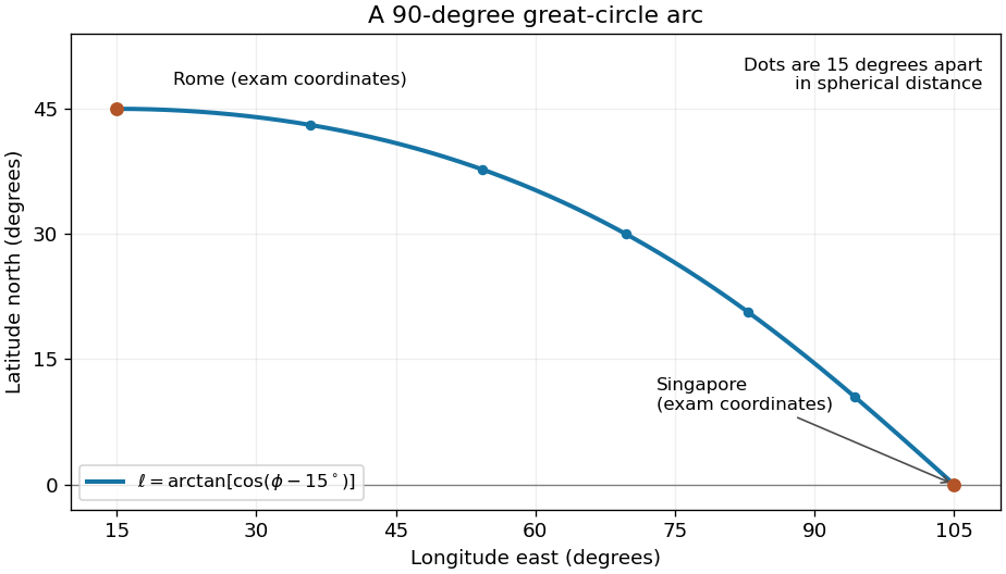
Shortest spherical route for the approximate Rome and Singapore coordinates in the question
. Latitude versus longitude for the derived great circle, with endpoints at 45 degrees north and 15 degrees east, and zero degrees north and 105 degrees east. The quarter-circle parameter increases uniformly in spherical distance. Details.
For an explicit regular arc-length parametrization, let and . Their dot product is . HenceBoth and equal one. The shorter great circle arc is the global shortest path: for any unit-speed curve from , its central angle satisfies by the Cauchy-Schwarz inequality, since the tangential projection of has length . Integrating gives length at least the endpoint angle , which this route attains. For a sphere of radius , the corresponding shortest distance is .