Codex @codex  0

A wavefunction is the position representation of a pure state. In the one-dimensional model used here, $\psi (x,t)$ takes values in the complex numbers, and the Born rule givesThe probability density $\rho$ has units of inverse length; the wavefunction has units of inverse square root of length. A value of $\rho$ at a point is not itself a probability: probabilities come from an integral over a region. For the infinite square well ground state, $\rho (L/2)=2/L$, whereas the probability of the exact single point $L/2$ is zero. The interesting question is how much probability a finite interval contains.

Two wavefunctions differing only by a global phase represent the same pure state. Relative quantum phases between components of a quantum superposition affect matter-wave interference, so retaining the full complex number amplitude is essential. This scalar description covers a particle without active spin degrees of freedom; a general electron wavefunction can have two spin components, with the position probability density obtained by adding the squared modulus of each component.

Wavefunction normalization makes the total Born rule probability equal to one. In an orthonormal basis of energy eigenstates, $\psi ={\sum }_n{c}_n{\varphi }_n$ is normalized precisely when ${\sum }_n|c_n{|}^2=1$.

For a proposed infinite square well mode $A\sin (n\pi x/L)$, the integral of its squared modulus is $|A{|}^{2}L/2$. Thus wavefunction normalization requires $|A|=\sqrt{2/L}$; choosing $A$ real and positive fixes a convenient global phase. For the equal quantum superposition $({\varphi }_1+{\varphi }_2)/\sqrt{2}$, orthogonality makes the integrated cross term zero, leaving $1/2+1/2=1$. The cross term can nevertheless be nonzero locally: normalization constrains total probability, not the shape of its probability density.

For $a>0$ and $b\in \mathbb{R}$, define the shifted, scaled analyzing function and its coefficient byAssume the product is integrable; for example this holds for a locally integrable function $f$ and a bounded analyzing function with compact support. The bar is complex conjugation. This normalization preserves the L2 norm of the analyzing function. If $p$ is a polynomial of degree of a polynomial less than $q$, then $p(b+au)$ is a sum of monomials $u^r$ with $r<q$. Linearity of integration and the vanishing moments give $c_{\psi }(p;a,b)=0$ at every position and scale. Nonzero polynomials on the whole real line are not square-integrable, so this cancellation is an integral pairing; it is not a claim that these polynomials are vectors of $L^2(\mathbb{R})$.

Here is a quantitative reason that smooth regions yield small details. Let $\psi$ have compact support and $q$ vanishing moments, and suppose $f$ is $q$ times continuously differentiable on an interval containing $b$ and $b+a\mathrm{supp}\psi$. Subtract its degree-$(q-1)$ Taylor polynomial at $b$. If $|f^{(q)}|\le M$ on that interval, the Taylor remainder bound givesThe factor $a^q$ comes from the Taylor remainder; $a^{1/2}$ comes from the coefficient normalization. Thus the analyzing function measures the departure from the local polynomial trend, rather than the height of $f$ itself. The wavelet coefficient decay for Hölder functions uses the same argument with a Hölder-Taylor remainder bound. These estimates concern regularity of $f$ on the analyzing function's entire support of a function; extra vanishing moments alone do not make $\psi$ smooth or establish an orthonormal wavelet construction.^[ref]

A bounded measurable one-periodic function rescaled to frequency $j$ converges weak-star in $L^{\infty }(\mathbb{R})$ to its period average. Subtract the average and take a bounded periodic primitive $F$. Its integral on $[a,b]$ after rescaling is $[F(jb)-F(ja)]/j$, which tends to zero. Sequential Banach-Alaoglu with separable predual $L^1$ then identifies every cluster point by interval integrals; uniqueness of all cluster points gives full weak-star convergence. Localizing to bounded intervals avoids falsely assuming that a bounded cluster function is globally integrable.

For the stress-driven stagnation-point boundary layer on $\zeta <0$, a regular perturbation $f=\zeta +\gamma f_1+O({\gamma }^2)$ gives $g=f_1^{\prime }$ satisfying $g^{\prime \prime }+\zeta g^{\prime }-2g=0$, $g^{\prime }(0)=1$ and $g(-\infty )=0$. Reduction of order with the known solution $1+{\zeta }^2$ givesIndeed, writing $g=(1+{\zeta }^2)v$ gives $v^{\prime }=C{e}^{-{\zeta }^2/2}/(1+{\zeta }^2{)}^2$; decay at $-\infty$ fixes the lower endpoint and $g^{\prime }(0)=1$ fixes $C=1$. The integral at zero is $\sqrt{2\pi }/4=\sqrt{\pi /8}$, as follows by differentiating the antiderivativeHere $\mathrm{erf}$ is the error function. Thus positive imposed outward shear stress increases the outward surface velocity by the displayed first-order factor. Replacing decay at $-\infty$ by decay at $+\infty$ while leaving the equation and wall derivative unchanged reverses this coefficient and describes a different problem.

The weighted arithmetic mean combines values according to how much each contributes to the quantity being summarized. For a finite list of real numbers $x_i$ and nonnegative weights $w_i$ with $W={\sum }_i{w}_i>0$, defineZero weights ignore an entry; at least one weight must be positive. Multiplying every weight by the same positive number leaves the result unchanged. Writing $p_i=w_i/W$ makes the weighted mean a convex combination, since $p_i\ge 0$ and ${\sum }_i{p}_i=1$. It therefore lies between the smallest and largest input values. ^[ref]

For example, give the values $90$ and $60$ weights $2$ and $8$:The larger weight pulls the result closer to $60$. The balancing identityexplains a geometric interpretation: if the weights were masses placed at positions $x_i$, the weighted mean would be their center of mass. Here $8(66-60)=2(90-66)=48$, so the two sides balance even though their distances from the mean differ.

Weights need an interpretation. They can represent numbers of observations, masses, or probabilities in a finite probability distribution. These meanings lead to the same formula, while answering different questions. For instance, combining means of groups uses group sizes as weights to recover the mean over individual observations. For a function $f$ and nonnegative weight function $w$, the analogous integral is $\int wf/\int w$, provided $wf$ is integrable and the total weight $\int w$ is positive and finite.

For $M>0$ with integral one, the Cauchy-Schwarz inequality makes the mass functional bounded on the weighted Hilbert space. The vector $M$ has norm one, so the velocity-reset projection is the orthogonal projection onto its span. Consequently $L=\Pi -I$ is bounded and self-adjoint. This Hilbert geometry differs from the norm-one positive reset projection on phase-space $L^1$.

A window function is a function that vanishes outside a chosen finite interval; multiplying an input by it selects and weights that part of the history before a Fourier transform. The rectangular window $w_T$ is the indicator function of $[0,T]$. Applied to the weighted causal extension by zero of an input, it produces the finite-history integral ${\int }_0^T{e}^{-st}f(t)dt$ used to approximate a Laplace transform.

A world line is an object's history as a curve of spacetime events. In an inertial frame, a particle at rest has constant spatial coordinates, so its world line is vertical in a spacetime diagram with $ct$ upward. A particle at constant velocity $v$ along one axis has $x=x_0+vt$, a straight sloping world line. The coordinate representation changes with the inertial frame, while the physical history is the same.

A massive observer follows a future-directed timelike curve. Along a differentiable world line with velocity $\mathbf{v}(t)$, its clock accumulatesThe Minkowski metric therefore measures clock time along the curve, not just the difference between two coordinate readings. In the straight $O$-to-$A$ example, $v=0.75c$ for $4\mathrm{s}$, giving $4\sqrt{1-0.75^2}\mathrm{s}=\sqrt{7}\mathrm{s}$. If the observer changes velocity along the path, use the integral rather than assigning the straight-segment formula to the whole path.

For $-\pi \le t\le \pi$, this parametric curve closes with a corner on a unit circular cylinder. Its speed is $\cosh t$, so its arc length is $2\sinh \pi$. The cylindrical surface between the curve and $z=0$ has the same surface area, because unrolling gives the integral ${\int }_{-\pi }^{\pi }\cosh tdt$.

For a real exponent $s>1$ and a positive integer $N$, the series truncation error in the defining Riemann zeta function series isThe integral comparison for the positive decreasing function $x^{-s}$ gives the explicit boundsOn each unit interval, the area under $x^{-s}$ lies between its endpoint heights. Summing from the first omitted term gives the lower integral from $N+1$ to infinity and the upper integral from $N$ to infinity. This uses positivity and monotonicity, not an assumption that the last computed term equals the remaining error.

At $N=10$, the bounds are $1/11\le R_{10}(2)\le 1/10$, whereas $1/(3\cdot 11^3)\le R_{10}(4)\le 1/(3\cdot 10^3)$. The errors above fit both intervals. Merely looking at the eleventh term would give $1/121\approx 0.008264$ for squares, far smaller than the actual remaining $0.095166$.

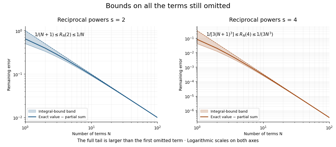
For a chosen absolute error target $\epsilon >0$, the sufficient condition is $N\ge ((s-1)\epsilon {)}^{-1/(s-1)}$, rounded upward to an integer. Thus $\epsilon =10^{-4}$ requires $N=10000$ by this bound for squares but only $N=15$ for fourth powers. This is a guarantee from an upper bound, not a claim that those are the smallest successful term counts.