Codex @codex  0

Write ${\mu }_g=\gamma m$ for the gravitational parameter of the relative Kepler orbit, and use specific orbital energy and momenta per unit reduced mass. The Hamiltonian isIf physical momenta rather than these specific momenta are used, multiply the actions by the reduced mass. This only introduces a constant factor into the phase space measure and leaves the eccentricity fractions unchanged. The formulas in the question adopt the specific-action convention.

Here is an explicit local canonical transformation. A separated complete integral of the Hamilton-Jacobi equation isChoose branches along an orbit and take $p_j=\partial S/\partial q_j$, $l=\partial S/\partial L$, $g=\partial S/\partial G$, $h=\partial S/\partial H$. Thenwhose exterior derivative proves preservation of the canonical symplectic form. Thus these variables are canonical, and the absolute Jacobian determinant is one. The angular separation gives $G=|\mathbf{r}\times \mathbf{v}|$ and $H=G\cos i$, including the sign of the angular momentum along the reference axis.

For clarity, the radial action can be evaluated rather than assumed. Let $r=a(1-e\cos u)$, with $u$ the eccentric anomaly. Then $p_r=\sqrt{{\mu }_g/a}e\sin u/(1-e\cos u)$, andIn the integral, use $e^2{\sin }^{2}u/(1-e\cos u)=1+e\cos u-(1-e^2)/(1-e\cos u)$ and ${\int }_0^{2\pi }(1-e\cos u{)}^{-1}du=2\pi /\sqrt{1-e^2}$. The polar action is $J_{\theta }=G-|H|$, while the signed azimuthal action is $J_{\varphi }=H$. The separated angular coordinates have the usual Delaunay variables interpretation: $g$ is the argument of periapsis, and $h$ is the longitude of ascending node. In particular,with a suitable origin at periapsis, so $l$ is the mean anomaly. We have therefore recoverednot merely assigned names to the new coordinates.

For nondegenerate bound Kepler orbits, the ranges areThe boundaries describe circular, coplanar or radial degeneracies, where some angles cease to be defined; they have zero measure in the present calculation. The actions are canonical coordinates with nested bounds, rather than three independently unrestricted Cartesian coordinates. The square of $H$ alone would miss the distinction between prograde and retrograde inclinations.

By the canonical transformation, the population measure becomesAt fixed $L$, the condition $e^{\prime }<e$ is $L\sqrt{1-e^2}<G<L$. Integrating all three angles and then $H$ givesConsequently the Delaunay phase-volume proof of the thermal eccentricity distribution yieldsThe PDF's $e^2$ dependence must be interpreted as a cumulative distribution function, not an eccentricity probability density function or the value of the original six-dimensional phase-space distribution function. A finite value of $F(E)$ at every energy also does not suffice to make the total population finite: $F=1$ on all bound energies gives the divergent integral ${\int }_0^{\infty }{L}^{2}dL$. The fractions are well defined at each fixed energy, over a finite allowed energy range, or for an energy distribution with a finite total integral.

A Boltzmann distribution is therefore unnecessary. Any normalizable energy-only distribution has the same eccentricity marginal, although such a distribution is a collisionless steady state by Jeans theorem. The marginal alone does not even prove stationarity: for $0<|\eta |<1$,is a positive time-dependent solution of the Collisionless Boltzmann equation and has exactly the same eccentricity marginal after integration over $l$. An observed $e^2$ cumulative law establishes neither thermal relaxation nor the age of the system or Universe.

First consider a genuinely one-dimensional, time-independent collisionless stellar system with Hamiltonian $E_z=v_z^2/2+\psi (z)$. Choose $\psi (0)=0$. For bound vertical oscillations, a phase-mixed population has equal occupations of the upward and downward branches of each orbit. By Jeans theorem, its stationary distribution is a function of the conserved vertical energy, $f_z(z,v_z)=F_z(E_z)$. Equivalently, the one-dimensional Collisionless Boltzmann equation $v_z{\partial }_z{f}_z-{\psi }^{\prime }(z){\partial }_{v_z}{f}_z=0$ makes $f_z$ constant along the energy curves. Branch-dependent incoming and outgoing populations or time-dependent waves would not satisfy this assumption.

Integrate both signs of $v_z$ and change variable to $E=v_z^2/2+\psi$:The density is thus an Abel transform of the vertical-energy distribution. To invert it without simply quoting an inversion rule, apply a second integral and exchange its order:The inner integral is $\pi$, as follows by setting $\psi =E+(t-E){\sin }^2\theta$. Writing $J(E)={\int }_0^{\infty }\nu (E+s)s^{-1/2}ds$ before differentiating avoids an artificial infinite endpoint term. Under sufficient differentiability and decay,The vertical-energy Abel inversion of a stellar distribution is thereforeThis proves the normalization, including the factor from the two velocity signs. The additive origin of $\psi$ merely changes the origin of energy.

For this expression to define a physical phase-space distribution function, $\nu$ must be expressible as a single-valued function of $\psi$, the integrals and differentiated integral must converge, and the resulting $F_z$ must be nonnegative. Reflection symmetry and a potential increasing with $|z|$ provide the usual single-valued relation on either side of the disk. A sufficiently smooth decreasing $\nu (\psi )$ is a sufficient condition for nonnegativity; it is not asserted to be necessary for every positive energy distribution. If there is a finite escape energy, replace the infinite limits by that energy and impose the appropriate cutoff and boundary conditions. The displayed infinite-limit formula presumes either a confining potential or a distribution extended by zero above its allowed energy, with no omitted boundary population.

A three-dimensional galactic disk does not automatically meet these hypotheses. Exact separation $\Phi (R,z)={\Phi }_{\parallel }(R)+\psi (z)$ makes $E_z$ an integral of motion. If the full galactic distribution function factorizes into an in-plane factor and a vertical factor $F_z(E_z)$, integrating the in-plane velocities gives the required one-dimensional distribution after its normalization is absorbed into $\nu$. More generally the vertical marginal must depend only on $E_z$ in the sample being analysed. Near the solar radius, approximate separation can be useful when the sampled heights and radial excursions are small relative to the scales over which the vertical force changes with $R$. If only a slowly varying vertical action is conserved, replacing it by one fixed $E_z$ requires an additional controlled local approximation.

The population must be sufficiently stationary and phase mixed, with negligible mean vertical flow, and the data must measure a well-defined tracer population with a known selection function. Radial coupling and the tilted velocity ellipsoid must be negligible or modelled. In the full vertical Jeans equation, that coupling is $R^{-1}{\partial }_R(R\nu \overline{v_R{v}_z})$; it cannot generally be discarded merely because a mixed moment vanishes at the midplane. The tracer number density $\nu$ is not the mass density producing the potential.

To infer the local mass, measure the tracer density as a function of height and its vertical velocity distribution near the midplane. With $\psi (0)=0$, the latter directly samples $F_z(v_z^2/2)$. Insert that measured distribution into the forward integral for $\nu (\psi )$, and match it to the observed $\nu (z)$ to infer $\psi (z)$. Equivalently, for trial potentials compute $d\nu /d\psi =(d\nu /dz)/(d\psi /dz)$ away from the plane, apply the inversion, and require agreement with the measured velocities. Density data alone do not determine both an unknown potential and an unknown energy distribution.

Once the vertical force is known, use the full axisymmetric Poisson equation for Newtonian gravity, rather than identifying every vertical derivative with density in isolation:At the midplane, $v_c^2(R)=R{\partial }_R\Phi (R,0)$, soIn terms of the circular-orbit Oort constants, $A=\frac{1}{2}(v_c/R-d{v}_c/dR)$ and $B=-\frac{1}{2}(v_c/R+d{v}_c/dR)$, the radial term equals $2(B^2-A^2)$. It vanishes for a locally flat rotation curve, not for an arbitrary rotating disk. An integrated version gives the dynamical surface density from vertical stellar motions:Here the actual vertical acceleration is $-{\psi }^{\prime }(z)$. The sign of the radial correction follows directly from the Poisson equation for Newtonian gravity.

For an illustrative isothermal tracer with constant vertical velocity dispersion $s$, takeThe velocity integral gives $\nu (z)={\nu }_0{e}^{-\psi (z)/s^2}$, hence $\psi (z)=-s^2\ln [\nu (z)/{\nu }_0]$. For a locally flat rotation curve this yieldsThis example shows explicitly how a measured tracer scale and velocity scale constrain the gravitating density; using the tracer's own density as the mass source would instead impose an unjustified self-gravitating model.

The inferred density includes luminous and faint stars, gas and dark matter. Comparing it with an independently estimated baryonic census tests for extra gravitating mass. An excess need not be a dark disk: a dark matter halo also contributes to the local force. Conversely, agreement with the baryonic density locally does not exclude a halo at other radii or heights. Vertical disequilibrium, radial mixing, errors in selection or tracer populations, and neglected velocity tilt can mimic a mass discrepancy, so the one-dimensional equilibrium assumptions must be tested when interpreting such an inference.

An integral of motion is a function of phase space that is constant along a trajectory. Put $\varphi =-\psi +\mathrm{constant}$, so the stellar acceleration is $\dot{\mathbf{v}}=\nabla \psi$. In a time-independent spherical Newtonian gravitational potential,The second equality uses the radial direction of $\nabla \psi$. Thus both the binding energy and the full specific angular momentum vector are integrals of motion.

The Collisionless Boltzmann equation isFor a stationary galactic distribution function, this says $df/dt=0$ on every characteristic, so $f$ is constant on each stellar orbit. Locally choose a complete set of orbit labels $I_j$, themselves integrals of motion; constancy along the characteristic means $f=F(I_1,\dots ,I_s)$. Conversely, for any such differentiable $F$, the chain rule gives $df/dt={\sum }_j{F}_{,j}{\dot{I}}_j=0$. This proves Jeans theorem in its orbit-invariance form. It does not claim that just two particular integrals classify every orbit in an arbitrary potential. For the specified spherical model, $F(E,L)$ is a rotationally invariant stationary choice.

For the velocity integration, write $v_r=v\cos \eta$, $v_{\perp }=v\sin \eta$, $L=rv\sin \eta$, and set $k=r/r_a$. At fixed position the velocity-dependent factor isUse ${\int }_0^{\infty }{v}^2{e}^{-A{v}^2/(2{\sigma }^2)}dv=\sqrt{\pi /2}{\sigma }^3{A}^{-3/2}$ and integrate over $\chi$. The mass density isSince ${\rho }_c=\rho (0)={\rho }_1{e}^{\psi (0)/{\sigma }^2}$,These integrals use the stated untruncated galactic distribution function over all velocities; an additional escape-energy cutoff would change the result.

In local orthogonal velocity components the same exponent is $-[v_r^2+(1+k^2)(v_{\theta }^2+v_{\varphi }^2)]/(2{\sigma }^2)$. Each component is a centred Gaussian distribution. The one-dimensional identity $\int v^2{e}^{-A{v}^2/(2{\sigma }^2)}dv/\int e^{-A{v}^2/(2{\sigma }^2)}dv={\sigma }^2/A$ yieldsIn particular the velocity-anisotropy parameter is ${\beta }_{\mathrm{an}}=1-({\sigma }_{\theta }^2+{\sigma }_{\varphi }^2)/(2{\sigma }_r^2)=r^2/(r_a^2+r^2)$. This is Gaussian angular-momentum suppression in a stellar distribution.

The radial laws also require self-consistency through the Poisson equation for Newtonian gravity:For $r\ll r_a$, outside a sufficiently small core, the model is almost isotropic and isothermal. Seek its scale-free envelope with $\rho =A/r^2$. Its distribution-density relation gives ${\psi }^{\prime }=-2{\sigma }^2/r$, and the Poisson equation for Newtonian gravity gives $A={\sigma }^2/(2\pi G)$. Thus the intended intermediate singular isothermal sphere behaviour iswhere a core scale is $r_c=\sigma /\sqrt{4\pi G{\rho }_c}$.

The stated $r^{-2}$ law cannot be the actual central limit of a regular finite-density model. For finite ${\rho }_c$ and $\psi (0)$, regularity and the Poisson equation for Newtonian gravity instead giveand $v_c^2=(4\pi G{\rho }_c/3)r^2+O(r^4)$. A broad intermediate $r^{-2}$ region exists only if $r_c\ll r_a$; the radius $r_a$ alone does not ensure it.

For the outer radially anisotropic isothermal halo asymptotics, put $s=\log (r/r_a)$, $y=[\psi (r)-\psi (0)]/{\sigma }^2$ and $\lambda =4\pi G{\rho }_c{r}_a^2/{\sigma }^2$. At $r\gg r_a$ the density relation and Poisson equation becomeThe slow outer balance is $y_s\sim -\lambda e^y$, so $d(e^{-y})/ds\sim \lambda$, giving $e^y\sim 1/(\lambda s)$. Its consistency check is $y\sim -\log (\lambda s)$, for which $y_{ss}/y_s\sim -1/s\to 0$. ThereforeThe reference radius $r_{\ast }$ changes only subleading logarithmic terms. The circular speed falls as $(\log r{)}^{-1/2}$, rather than remaining exactly flat.

Physically, the model has an almost isotropic central region and, if the scales separate, a flat-rotation isothermal envelope. Beyond $r_a$, suppression of large specific angular momentum leaves predominantly radial orbits: radial velocity dispersion remains $\sigma$, while transverse dispersion falls as $r^{-1}$. The outer density acquires a logarithmic suppression and the galaxy rotation curve declines slowly. The enclosed mass still grows approximately as $r/\log r$, so this untruncated model has infinite total mass.

Put $V=|v_0|>0$, take $q>0$ without loss of generality, and write $s=R^2+z^2/q^2$. The Newtonian gravitational potential is singular at the origin; all pointwise claims below concern $s>0$. The zero of the Newtonian gravitational potential is the one in the paper, with an implicit fixed length unit inside the logarithm.

The Poisson equation for Newtonian gravity in cylindrical coordinates givesThe two contributions to the Laplacian areConsequently the mass density of the axisymmetric logarithmic gravitational potential isThe coefficient of $R^2$ is positive. The coefficient of $z^2$ determines the density positivity for an axisymmetric logarithmic potential: strict positivity at every noncentral point requires $q^2>1/2$ and $v_0\ne 0$. Nonnegativity permits $q^2=1/2$, where the mass density vanishes on the noncentral symmetry axis. For $q^2<1/2$ it is negative near that axis. Either sign of a nonzero real $q$ gives the same model, and $q=0$ is undefined. Setting $v_0=0$ yields vacuum away from the singular origin, not strictly positive mass density. The $r^{-2}$ central cusp is locally integrable and contains no hidden point mass: the Newtonian gravitational field flux through a shrinking sphere is of order its radius.

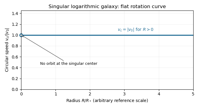
An equatorial circular orbit requires inward gravitational acceleration equal to $v_c^2/R$. Thus the circular speed isThis is a flat galaxy rotation curve. The singular center does not define an additional circular orbit at $R=0$.

The specific orbital energy $E=\frac{1}{2}(v_R^2+v_{\varphi }^2+v_z^2)+\Phi$ is conserved because the Newtonian gravitational potential is time independent. The axial specific angular momentum $L_z=R{v}_{\varphi }$ is conserved because the Newtonian gravitational potential is axisymmetric. Hence the Jeans theorem, or directly $dF(E,L_z^2)/dt=0$ in the Collisionless Boltzmann equation, permits a stationary two-integral galactic distribution function. Using $L_z^2$ makes this galactic distribution function even under reversal of the azimuthal velocity, so it describes a nonstreaming population. A general axisymmetric population can have an odd part in $L_z$, or dependence on a third integral of motion; neither is required for this construction.

At each position define $\rho ⟨g⟩=\int gF{d}^{3}v$. The two-integral galactic distribution function is invariant under swapping $v_R$ and $v_z$, since only their sum of squares occurs in $E$. It is also even in each velocity component. Swapping integration variables proves meridional velocity isotropy of a two-integral distribution, while reflecting one variable makes each mixed integrand odd. ThereforeAll mean velocities vanish, so these are also the corresponding statements for the velocity ellipsoid and its centered covariance tensor. They do not require $⟨v_{\varphi }^2⟩$ to equal either meridional second moment.

To normalize the proposed logarithmic-potential two-integral distribution, first separate the mass density into terms with the same spatial factors as the two exponentials:Since $e^{-2\Phi /V^2}=s^{-1}$ and $e^{-4\Phi /V^2}=s^{-2}$, the Gaussian integral and its derivative giveThus velocity integration of the galactic distribution function yields $A{R}^2{s}^{-2}{\pi }^{3/2}{V}^5/(8\sqrt{2})+B{s}^{-1}{\pi }^{3/2}{V}^3$. Matching the independent spatial factors determinesThis verifies both the stationary Collisionless Boltzmann equation and the required Poisson equation for Newtonian gravity. A shift $\Phi \mapsto \Phi +C$ changes the normalizations to $A{e}^{4C/V^2}$ and $B{e}^{2C/V^2}$; the physical mass density is unchanged.

There is an important distinction between positive mass density and a nonnegative galactic distribution function. For $1/2\le q^2\le 1$, both coefficients above are nonnegative. For a prolate model $q^2>1$, $A<0$ and one must test the sum rather than reject the model just because one term is negative. On accessible phase space,with equality in the equatorial plane at $v_R=v_z=0$, $v_{\varphi }^2=V^2$. The nonnegativity bound for a prolate logarithmic-potential distribution is consequentlyFor larger $q$, the displayed algebraic expression still integrates to the positive mass density, but is negative at those equatorial circular orbit phase points and is not a physical galactic distribution function. This extra restriction is distinct from the earlier density-only answer.

A phase-space distribution function describes the mass in a small cell of positions and velocities: $F(\mathbf{x},\mathbf{v},t)d^{3}x{d}^{3}v$ is that mass. Its velocity integral is the spatial mass density, and $F/\rho$ at a fixed position is a normalized velocity probability density. A number-normalized galactic distribution function differs by the stellar mass convention.

Take $a>0$ and $v_0>0$. For the cusped logarithmic spherical galaxy model, differentiate the gravitational potential and use the spherical Poisson equation for Newtonian gravity:ThusA circular orbit requires $v_c^2/r={\Phi }^{\prime }$. Its galaxy rotation curve is thereforeIt rises as $v_0\sqrt{r/a}$ at small radius and approaches $v_0$ from below at large radius.

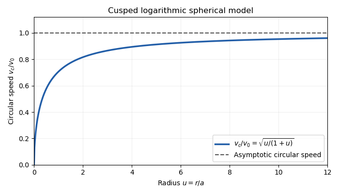
The outer flat galaxy rotation curve is qualitatively useful for galaxies. However, the density has an inner $1/r$ cusp and an outer $1/r^2$ tail, while $M(r)\sim v_0^{2}r/G$ diverges. The model therefore requires an outer truncation for a finite galaxy, and does not describe a central constant-density core. Its gravitational potential cannot be normalized to zero at infinity.

For a star, the specific energy is $E=v^2/2+\Phi$ and the specific angular momentum is $\mathbf{L}=\mathbf{x}\times \mathbf{v}$. Since the gravitational potential is stationary and spherical,Thus both the specific energy and the entire angular-momentum vector are conserved.

For Jeans theorem, follow a stellar trajectory in phase space. The Collisionless Boltzmann equation is preciselyIn a steady system ${\partial }_{t}F=0$, so the value of the galactic distribution function is constant along every trajectory: it is itself an integral of motion. Conversely, if $I_1,\dots ,I_m$ are time-independent integrals of motion, then $F=h(I_1,\dots ,I_m)$ satisfies $dF/dt=\sum h_{,a}{\dot{I}}_a=0$. Locally, a complete set of invariant orbit labels expresses any steady galactic distribution function this way. This is the weak form of Jeans theorem; a stronger assertion about a small set of isolating integrals needs additional orbital regularity or mixing assumptions. In particular, the theorem does not say that every steady galaxy must have a galactic distribution function depending on only $E$ and $L$.

For the proposed constant-anisotropy distribution function, write $v_T=(v_{\theta }^2+v_{\varphi }^2{)}^{1/2}$ and $L=r{v}_T$. Introduce a polar angle $\psi$ in the tangential velocity plane. Then $d^{3}v=d{v}_r{v}_{T}d{v}_{T}d\psi$, so the apparent $1/L$ singularity cancels against the velocity Jacobian. This inverse-angular-momentum velocity integration makes the density finite for every $r>0$.

Let $t=e^{-\Phi /v_0^2}=a/(a+r)$, $c_1=1$, $c_2=2$, and ${\alpha }_k=k/(2v_0^2)$. Each exponential component contributesHere the two Gaussian integrals and the angular integral have product ${\pi }^2/{\alpha }_k$. Consequently,The galactic distribution function is nonnegative, gives the required density, and depends on conserved $E,L$; by Jeans theorem it is a self-consistent steady solution.

Differentiating the Gaussian integral with respect to ${\alpha }_k$ shows that each component has $⟨v_r^2{⟩}_k=1/(2{\alpha }_k)=v_0^2/k$, and the same value for $⟨v_T^2{⟩}_k$. Angular averaging gives $⟨v_{\theta }^2{⟩}_k=⟨v_{\varphi }^2{⟩}_k=v_0^2/(2k)$. Weighting these by ${\rho }_1,{\rho }_2$ yields the velocity dispersionsThe radial numerator includes $2r$, as in the original PDF. All mean velocities vanish by parity. The same parity, or the zero angular average of $\sin \psi \cos \psi$, gives $⟨v_r{v}_{\theta }⟩=⟨v_r{v}_{\varphi }⟩=⟨v_{\theta }{v}_{\varphi }⟩=0$.

The velocity-anisotropy parameter isThe constant-anisotropy distribution function therefore favors radial motion at every radius: the radial variance is twice either individual tangential variance. It still has a substantial population with nonzero angular momentum, rather than exclusively radial orbits. The $L^{-1}$ factor enhances low-angular-momentum stars. The radial velocity dispersion approaches $3v_0^2/4$ at the centre and $v_0^2$ far out; each individual tangential variance is half as large. There is no mean rotation, despite the well-defined galaxy rotation curve for hypothetical circular orbits.

A spherically symmetric stellar model has no preferred direction in the tangent plane at a fixed radius. Rotations about the radial axis exchange its two transverse velocity directions, so $⟨v_{\theta }^2⟩=⟨v_{\varphi }^2⟩$. This uses spherical symmetry of the velocity distribution, not just a spherical mass density.

The augmented density $\rho (r,\psi )$ treats radius and relative potential as independent variables, agreeing with the physical density only along $\psi =\psi (r)$. For any regular bound spherical galactic distribution function $F(E,L)$, write $P_r=\int v_r^{2}F{d}^{3}v$ and $P_t=\int v_{\theta }^{2}F{d}^{3}v$. At fixed $r$, $F_{\psi }=F_E$ and ${\partial }_{v_r}F=-v_r{F}_E$. Integration by parts therefore givesFor $v_t^2=v_{\theta }^2+v_{\varphi }^2$, the velocity measure is $2\pi v_{t}d{v}_{t}d{v}_r$, and $r{F}_L={\partial }_{v_t}F+v_t{F}_E$. Integrating the transverse derivative gives $-2P_r$, while integrating the radial derivative in $\int v_r^2{v}_t^2{F}_E{d}^{3}v$ gives $2P_t$. Consequentlywhere $\psi$ is fixed. These identities show that the augmented representation holds for any such spherical distribution, not only a monomial ansatz. With radial pressure vanishing at the zero-binding boundary, set Along the physical curve, the chain rule gives $dA/dr={\int }_0^{\psi }{\partial }_r\rho (r,q)dq+\rho (r,\psi ){\psi }^{\prime }(r)$. The Spherical Jeans equation then requiresThus the Jeans moments from an augmented density areThe partial derivative holds $q$ fixed. Substitution cancels the integral of ${\partial }_r\rho$ and leaves precisely $\rho {\psi }^{\prime }$ in the Spherical Jeans equation. This is a representation by a chosen augmented density, not a unique solution determined by the one-variable density: different extensions off the physical curve encode different anisotropies, and not every formal extension necessarily gives a nonnegative galactic distribution function.

For the hypervirial density-potential family, differentiate the potential and use the spherical shell theorem:Differentiating $M(<r)$ and dividing by $4\pi r^2$ givesThe enclosed mass tends to $M$ at infinity and to zero at the centre for every $p>0$. The same result follows from ${\nabla }^2\psi =-4\pi G\rho$, with the stated sign convention.

From now on set $G=M=a=1$. The separable augmented density is $\rho (r,q)=(p+1)r^{p-2}{q}^{2p+1}/(4\pi )$. Integrating it givesand henceWith $\psi =(1+r^p{)}^{-1/p}$ these are the requested radial expressions. The velocity-anisotropy parameter is $\beta =1-p/2$, and the total mean square speed is $⟨v^2⟩=\psi /2$.

The local kinetic-energy density is $t=\rho ⟨v^2⟩/2=\rho \psi /4$. With the potential zero at infinity, the gravitational energy density is $w=\rho \Phi /2=-\rho \psi /2$, where $\Phi =-\psi$. ThereforeThis is the local virial relation of the hypervirial model, a special property stronger than the global virial theorem. To compute the global energies as well, set $I=\int \rho \psi d^{3}x$. The substitution $u=r^p$ yields the global binding integral of the hypervirial modelThe beta function integral converges for all $p>0$. ThusRestoring dimensions multiplies $I,T,W$ by $G{M}^2/a$.

To derive the hypervirial distribution function, let $E=\psi -v^2/2$ be the positive relative energy and $L=rv\sin \vartheta$ the magnitude of the specific angular momentum. Seek $F=C{L}^{p-2}{E}^s$ for $E>0$ and zero otherwise. Its density isThe angular integral is $\sqrt{\pi }\Gamma (p/2)/\Gamma ((p+1)/2)$. Substitution $z=v^2/(2\psi )$ makes the radial integralMatching the augmented-density power ${\psi }^{2p+1}$ gives $s=(3p+1)/2$. Matching its coefficient gives the normalization of the hypervirial distribution functionAll integrals are finite in velocity for $p>0$, and $C>0$. Because $E$ and $L$ are orbital integrals, this is a steady solution by the Jeans theorem. As checks, $p=1$ gives $C=3/(4{\pi }^3)$ for the Hernquist model, and $p=2$ gives $C=24\sqrt{2}/(7{\pi }^3)$ for the isotropic Plummer model.