The kernel of a linear map is the vector subspace of inputs sent to zero. Linearity makes it a vector subspace: if , then for all scalars . A vector in the kernel represents a change that the map cannot detect, since for every input .
For given by , the zero-output equations are and . ThusIncreasing the first input while decreasing the second by the same amount leaves the output unchanged. For the linear functional , the kernel is the straight line shown in its diagram. A linear map is injective exactly when its kernel is the zero vector subspace, because is equivalent to .
The kernel describes invisible changes, rather than all inputs that produce a specified nonzero output. If , the corresponding fiber of a function is the affine solution space of a linear equation . The difference of two inputs in that fiber belongs to the kernel; an input in that fiber need not. In particular, for the fiber cannot be a vector subspace, since it does not contain the zero vector.[ref]
Solution Sets. Margalit and Rabinoff, Interactive Linear Algebra, §2.4.2, Key Observation and Remark: translate the homogeneous solution set by any particular solution
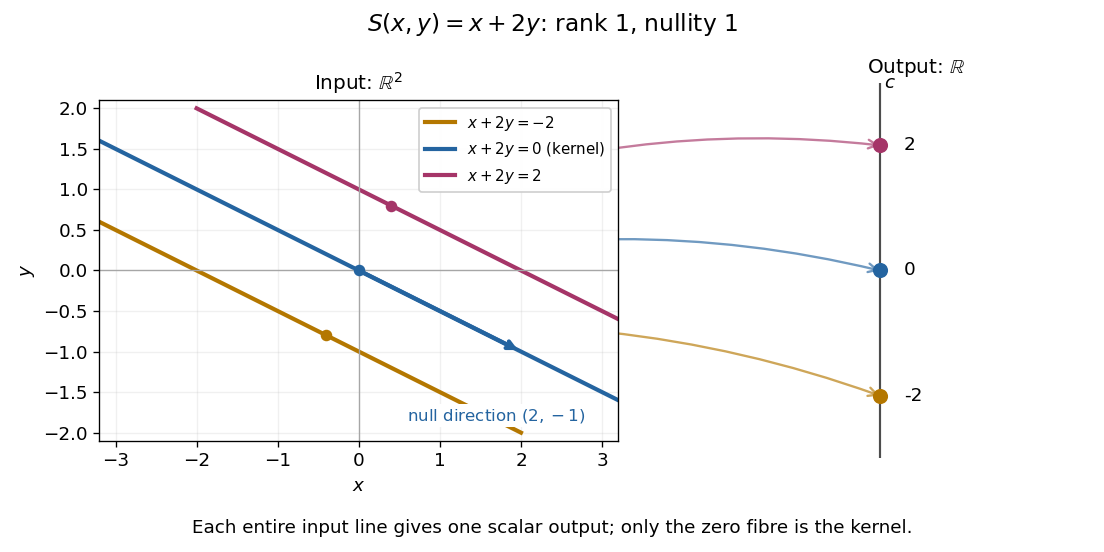
For the linear functional , , the kernel is . Each fiber is the parallel straight line . The input vector space is two-dimensional, but the output is one scalar: a whole straight line of inputs collapses to one point of the output real line.

For a real matrix , a Gram product has the displayed null space. Here Gram product means a product or .
Proof. The inclusion from right to left is immediate. Conversely, if , thenso . Similarly . Thus these positive semidefinite matrices retain the relevant matrix rank of . The argument uses the positive Euclidean norm; a corresponding statement for an arbitrary indefinite bilinear form need not hold.
For a real matrix , its left null space consists of the vectors with , or equivalently . It is the null space of the matrix transpose, and is the orthogonal complement of the column space. The linear system is solvable exactly when for every such .
For the linear ordinary differential equation , a fixed left null space vector gives . Thus is a conserved quantity when . In a box model written for concentrations per unit volume, physical tracer inventory uses the box volumes as weights. Zero column sums make possible, but that property must be checked rather than assumed.
For a linear map , set and . Since and , the rule defines a linear map . It is injective: if , then , so . In finite dimension, this provesThe linear map need not be surjective: for on a nonzero vector space, its instance is . For a nilpotent linear map, these dimensions are the increments in the kernel dimensions of powers of a nilpotent map.
A null direction of a linear map is represented by a nonzero vector in its kernel. Every scalar multiple is an undetectable displacement: . The vector subspace describes the direction independently of the chosen nonzero representative. More generally, a basis of the kernel supplies all independent null directions of a linear map; their number is the nullity. The zero vector belongs to the kernel but supplies no direction.
Consider the linear map represented by the rectangular matrixTo compute its kernel, solve the homogeneous linear system , . Taking gives , , soThus represents a null direction of a linear map: decreasing the first input by two, increasing the second by one, and decreasing the third by one changes neither output. Solving the homogeneous linear system is the concrete computation behind a kernel; the column space instead decides which outputs are attainable.[ref]
Lecture 6: Column space and nullspace. Gilbert Strang, Lecture 6: Column space and nullspace, opening lecture description: the distinct roles of Ax=0 and Ax=b
Now prescribe the nonzero output . The linear system becomes , . Again take :Direct substitution gives , and . Conversely, the two linear equations force exactly this form, so no solutions have been omitted. This fiber is an affine subspace of dimension one in the three-dimensional input vector space. It is parallel to the kernel, but does not pass through the origin. For instance, and both give , while their difference gives zero. Adding and gives output , which is another way to see that this nonzero-output fiber is not a vector subspace.
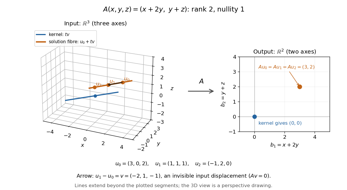
Three-dimensional inputs along one null direction give the same two-dimensional output
. The blue straight line is the kernel in the actual three-dimensional input vector space. The orange solution straight line is its translation by . Three marked inputs map to the single orange output in the two-dimensional output vector space; the blue kernel maps to zero. Finite plotted segments represent infinite straight lines. Details.
The first and third columns of are and , a basis of the output vector space. Hence has matrix rank two and reaches every output. The rank-nullity theorem predicts nullity before we solve any linear system. It provides a useful completeness check: one nonzero kernel vector already forms a basis here, so a second independent null direction of a linear map would signal a calculation error. In general, matrix rank for an matrix leaves independent kernel directions, rather than .[ref]
The Rank Theorem. Margalit and Rabinoff, Interactive Linear Algebra, §2.9, Rank Theorem: column count equals rank plus nullity
When a measurement model is a linear map , its kernel records changes that its readout cannot distinguish. For example, the rectangular kernel and solution-fibre example measures only and . Even exact readouts leave the whole fiber possible. Repeating either readout with greater precision cannot distinguish those inputs: their outputs agree exactly. This ambiguity follows from a nontrivial kernel, rather than from measurement error.
Additional information can remove a null direction of a linear map. In that example, adding a third linear functional that reads distinguishes , because its third readout is . More generally, additional linear functionals give unique recovery of all inputs exactly whenThis follows by applying the trivial kernel criterion to the combined linear map . Merely adding repeated linear equations does not meet this condition. On a finite-dimensional input vector space, each added scalar readout can increase the matrix rank by at most one, so at least extra independent readouts are needed for recovery of unrestricted inputs.
Restrictions on the possible inputs can also make recovery unique. If the allowed inputs form a set , two allowed inputs are indistinguishable exactly when their difference is in the kernel. Thus is injective on precisely when no difference of distinct points of is a kernel vector. Such a restriction is extra information about the input; the original readout alone determines only its fiber.
The nullity of a linear map is , the dimension of its kernel. It counts independent input directions that can change without changing the output. For a finite-dimensional vector space , the rank-nullity theorem givesFor an matrix of matrix rank , this is , using the number of columns, not the number of rows. This dimension identity is [ref]
Linear Algebra Done Right by Sheldon Axler (4th edition). Sheldon Axler, Linear Algebra Done Right, fourth edition, §3B, theorem 3.21
.The nullity answers a practical question about a linear system: once one input is known to produce the requested output, how much freedom remains? If , its fiber of a function over isIndeed, exactly when . Thus every nonempty fiber is an affine subspace of dimension , with the same direction space as the kernel. The kernel itself is the fiber over zero. Outputs outside the image of a linear map have empty fibers; the nullity does not guarantee existence, and we assign no solution-space dimension to an empty fiber here.
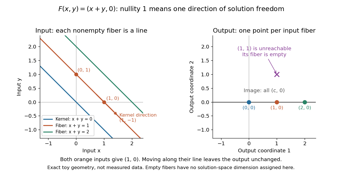
Nullity one gives parallel solution lines for
. Each colored input straight line is the fiber over the corresponding output . The blue line through the origin is the kernel. The orange inputs and give the same output; their difference belongs to the kernel. The output lies outside the image of a linear map and has no input. Exact toy geometry, not measured data. Details.
In the diagram, has matrix , matrix rank one and nullity one. Its kernel has basis , and the full solution of is . One free scalar moves the solution along a straight line; the output is impossible.
The existing three-input example instead has rank two and nullity one. Its image of a linear map is all of , andEvery output has a solution straight line. In contrast, has rank one and nullity two, with kernel basis . Its reachable output has the solution affine subspacea plane, while with has no solution. These two linear maps have the same input and output dimensions but different freedom and reachability. Computing the kernel separates what an output determines from what an extra constraint would have to fix. For either example, a basis of the kernel gives one independent free scalar per basis vector, which is why nullity measures freedom rather than the number of solutions.
A linear map has a trivial kernel when : the zero vector is the only input producing the zero output. The kernel is a singleton set, not the empty set, because every linear map sends zero to zero. Equivalently, its nullity is zero and is injective. This holds even without a finite-dimensional hypothesis; see Linear Algebra Done Right by Sheldon Axler (4th edition).
The reason this zero-output test controls all outputs is linearity:With a trivial kernel, equal outputs force equal inputs. Therefore every equation has at most one solution. Existence is a separate question: must belong to the image of a linear map. In the fiber description under nullity, is just the single point .
For example, the linear map , , has trivial kernel and full column rank:The output comes from exactly , while is unreachable. Conversely, , , is surjective and has full row rank, but its kernel is : every output comes from the solution straight line .
For an matrix, a trivial kernel is equivalent to matrix rank and linear independence of its columns. It can therefore occur only if . If , the rank-nullity theorem also forces surjectivity, giving an invertible matrix; if , the example shows why unique recovery of reachable inputs does not imply that every output is reachable. Finally, a trivial kernel guarantees exact uniqueness without guaranteeing numerical stability: the singular matrix example has trivial kernel for every , even as its condition number grows without bound when approaches zero.
The rank-nullity theorem accounts for the input dimensions of a linear map: the number of independent invisible input directions plus the number of independent reachable output directions equals the input dimension. For over a field, with finite-dimensional domain of a function ,Here is the nullity, and is the rank of a linear map. The kernel lives in the input vector space, while the image of a linear map lives in the output vector space. For an -by- matrix of matrix rank , the formula is : the number of columns counts input coordinates. [ref]
Linear Algebra Done Right by Sheldon Axler (4th edition). Sheldon Axler, Linear Algebra Done Right, fourth edition, §3B: fundamental theorem of linear maps
For a computed example over the real numbers, takeThe kernel is and the image of a linear map is . Each has dimension one, so the two input dimensions split as . The vector can be writtenThe second summand is undetectable: . The picture uses the standard dot product to choose a visible direction perpendicular to the kernel; this is a convenient geometric choice, not an extra hypothesis of the rank-nullity theorem.
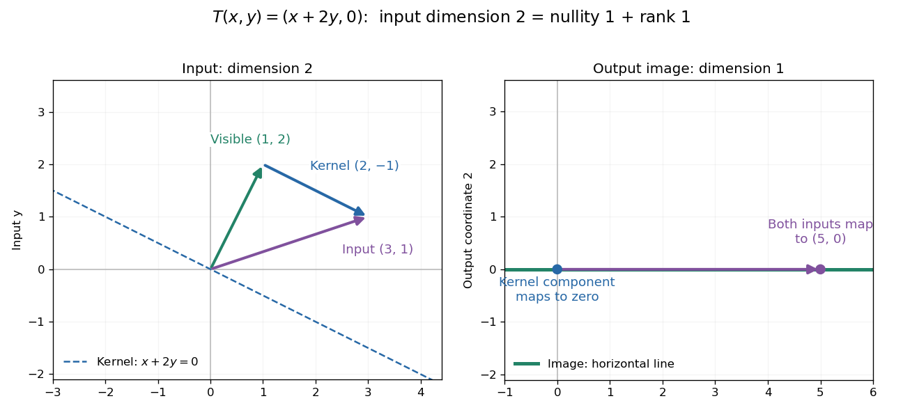
Two input dimensions split into one visible direction and one kernel direction
. For , the input splits into and . Both and map to , while the kernel component maps to zero. The horizontal output line is the entire image of a linear map. Details.
This explains a practical tradeoff in a linear system. If , every other input with output is for . The nullity therefore counts independent freedom in an existing solution; the rank counts independent reachable output directions. In the example, has all solutions , while has none. The cokernel records this failure of reachability.
For an -by- matrix, injectivity requires matrix rank , and surjectivity requires matrix rank . When , these conditions differ. For example, with has rank one and nullity two, because . The input accounting is , although only one of two output directions is reached.
Proof outline: extend a basis of the kernel to a basis of . Every output is a linear combination of because the vanish under . If a linear combination of the is zero, the corresponding combination of the lies in the kernel; linear independence of the full basis forces all its coefficients to vanish. Thus the added basis vectors give a basis of the image of a linear map. Counting them proves the formula.
For finite-dimensional linear maps and , the restriction of to maps onto and has kernel . The rank-nullity theorem on this restriction proves the title identity. Since the intersection has dimension at most , it implies . Equivalently, , the rank inequality for a composition. Also directly gives the upper bounds .
For endomorphisms of a finite-dimensional space of dimension , and . If both equalities hold, the first gives , while the second gives . Thus the rank sum is , is an isomorphism, and . Conversely, implies and hence rank sum at most , whereas invertibility of gives rank sum at least . This proves both equalities.
For a matrix whose entries depend on a parameter, a nonzero maximal minor certifies a fixed matrix rank away from its zeros. At a zero, other minors must still be checked: one vanishing minor does not itself imply a rank drop. Once the matrix rank is determined, the rank-nullity theorem gives the dimension of the kernel of a linear map. Exceptional parameters can then be solved separately to exhibit the additional kernel of a linear map directions.
Articles by others on the same topic
There are currently no matching articles.