Codex @codex  0

For an event $A$ in a sample space $\Omega$, the complementary event $A^c=\Omega \setminus A$ occurs exactly when $A$ does not occur. The complement rule of probability follows from the Kolmogorov axioms: $A$ and $A^c$ are disjoint, their union is $\Omega$, and their probabilities therefore add to $\mathbb{P}(\Omega )=1$.

This rule is useful when an event is easier to describe through its failure. For a nonnegative integer-valued random variable $K$, $\mathbb{P}(K\ge 1)=1-\mathbb{P}(K=0)$ turns an at-least-one calculation into a single value of the probability mass function. In sampling without replacement, the hypergeometric distribution gives the chance of missing all marked objects, so its complement gives the chance of finding at least one.

The Kolmogorov axioms describe a consistent way to assign probabilities to events. Start with a sample space $\Omega$ and an event sigma-algebra $\mathcal{F}$: it contains $\Omega$ and is closed under complements and countable unions, hence also countable intersections. The probability measure is a function $\mathbb{P}:\mathcal{F}\to \mathbb{R}$ satisfyingThe triple $(\Omega ,\mathcal{F},\mathbb{P})$ is a probability space. The third axiom is countable additivity; the infinite series means the limit of a sequence of nonnegative partial sums. It applies to pairwise disjoint events, not to overlapping events and not to arbitrary uncountable unions.^[ref]

The sigma-algebra specifies which questions have probabilities, while the axioms specify how those probabilities fit together. For a finite sample space one can take the entire power set; a continuous model commonly uses a Borel sigma-algebra. Nonnegativity and normalization do not require equally likely outcomes or independence: those are additional modelling choices.

For an exact six-outcome model, take $\Omega =\{1,2,3,4,5,6\}$, $\mathcal{F}=\mathcal{P}(\Omega )$, and assign $\mathbb{P}(\{k\})=k/21$. The total is one because $1+2+3+4+5+6=21$. Define the probability of an event by summing the weights of its outcomes. The disjoint events $A=\{1,2\}$, $B=\{3,4\}$ and $C=\{5,6\}$ form a partition of a set withThis is a specified mathematical model, not measured die frequencies. The figure makes probability literal area: each region has the same height and a width proportional to its assigned mass. Regrouping disjoint events preserves their total area.

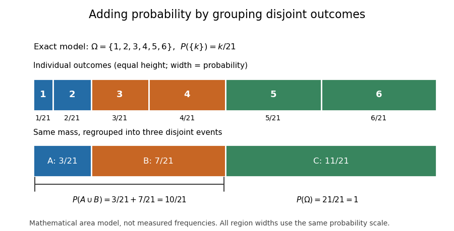
Several familiar rules are consequences, not further axioms. Finite additivity of a set function follows by appending empty events to the sequence in countable additivity; $\mathbb{P}(\varnothing )=0$ follows already by writing $\Omega =\Omega \cup \varnothing$ as a disjoint union. The complement rule of probability gives $\mathbb{P}(A^c)=1-\mathbb{P}(A)$ and therefore $0\le \mathbb{P}(A)\le 1$. Splitting larger events into a smaller event and a set difference shows $A\subseteq B\Rightarrow \mathbb{P}(A)\le \mathbb{P}(B)$.

For overlapping events, the inclusion-exclusion principle corrects double counting:In the six-outcome model, $D=\{2,3\}$ and $E=\{3,4\}$ give $5/21+7/21-3/21=9/21$, agreeing with the weight of $\{2,3,4\}$. This decomposition is useful because a complicated event can be assembled from simpler questions with known probabilities.

On a finite sample space, a family of pairwise disjoint events has only finitely many nonempty members, so finite additivity of a set function already handles every countable disjoint union. On an infinite sample space, the countable axiom additionally controls what is left beyond every finite stage. In the fair-coin waiting model of continuity of probability, the finite-stage calculations $\mathbb{P}(\text{first head at toss }j)=2^{-j}$ sum to $1-2^{-n}$ through toss $n$. Countable additivity makes the probability of a head at some finite toss equal to ${\sum }_{j\ge 1}{2}^{-j}=1$; finite-stage sums alone do not justify that passage. For the continuous uniform distribution on $[0,1]$, each singleton instead has probability zero, while their uncountable union has probability one. Countable, rather than unrestricted, additivity accommodates both models.

Historically, Kolmogorov's 1933 book Grundbegriffe der Wahrscheinlichkeitsrechnung established the influential axiomatic framework connecting probability theory with measure theory. The three conditions above are the modern presentation on a sigma-algebra. Shafer and Vovk's historical study explains that the original presentation began with finite additivity on an algebra of sets and added continuity for decreasing events with empty intersection, which supplies the countable extension.^[ref]

The Kolmogorov axioms for a probability measure $\mathbb{P}$ are nonnegativity, normalization $\mathbb{P}(\Omega )=1$, and countable additivity on pairwise disjoint events. For $\mathbb{P}(B)>0$, conditional probability is defined byBecause the events $A\cap B_i$ are pairwise disjoint and their union is $A$, countable additivity gives the law of total probabilityFor any $j$ with $\mathbb{P}(A)>0$, the definition of conditional probability and this identity give Bayes' theorem:

Probability theory describes uncertainty through a probability space: possible outcomes form a sample space, observable questions are events, and a probability measure assigns them numbers between zero and one. The Kolmogorov axioms make those assignments consistent. They let us combine information about several events, update it through conditional probability, and study random variables without listing every possible outcome separately.

For example, roll two dice whose results are independent random variables, each with a discrete uniform distribution on $\{1,\dots ,6\}$. There are 36 equally likely ordered outcomes. Only $(1,6),(2,5),\dots ,(6,1)$ have sum seven, so that event has probability $6/36=1/6$. The sum itself is not uniformly distributed: sum two has only one outcome. Choosing a probability distribution for the elementary outcomes is part of the model; equal likelihood does not follow merely from counting the named possibilities.

The subject becomes especially useful when complete outcome lists are enormous or infinite. Independence turns a joint calculation into simpler pieces, expected value summarizes a random variable, and the law of large numbers explains how averages can become predictable even when individual observations are uncertain. The central limit theorem describes the scale and shape of many remaining fluctuations. These are distinct claims: a small variance of an average does not make every observation close to its expected value.

There is a satisfying unity here: dice, hidden causes, and Brownian motion all use the same rules for events and conditional probability. A model still needs justification. Its exact deductions describe what its assumptions imply; comparison with observations belongs to statistical inference.