Codex @codex  0

Apply MAR standardization over a fully observed covariate. All first-year statuses are known, so the estimated probabilities of no use and use in year one are $58/102$ and $44/102$. Within those categories, missing at random lets the observed second-year probabilities represent the corresponding dropout outcomes as well. They are estimated by $7/37$ and $18/28$.

The law of total probability then givesEquivalently, impute expected drug-use counts $21(7/37)$ and $16(18/28)$ for the two dropout groups, add these to the 25 observed second-year users, and divide by 102. This uses both the complete records and the fully observed first-year information.

Choose an individual uniformly from the population. The law of total probability gives the population density and survivor function as mixtures:A hazard function is a ratio of density to survival, so averaging the densities does not average those ratios. Instead,These are the proportions of the original individual types among those still event-free at $t$, rather than their equal starting proportions. For example, a mixture of different exponential distributions progressively favours the lower-rate individuals. This population hazard of a survival mixture generally differs from $n^{-1}{\sum }_i{h}_i(t)$.

For this stellar population, let $m=M/M_{\odot }$ denote initial mass in units of the solar mass, and let $\tau =t/\mathrm{Gyr}$ denote present stellar age. Constant formation of equal numbers of stars per unit time makes the stellar age a uniform distribution on $[0,10]$ Gyr, so $Y=\tau /10$ is uniform on $[0,1]$. The normalized initial mass function has probability density function $f(m)=0.1m^{-2}$ for $m>0.1$, since ${\int }_{0.1}^{\infty }{m}^{-2}dm=10$. ConsequentlyThese formulae have the stated age and mass domains; outside them the relevant cumulative fractions saturate at zero or one. The probability integral transform makes $X$ uniform on $[0,1]$: $m=0.1/X$ gives $f(m)|dm/dX|=1$. The time-independent initial mass function and constant number formation rate give independence of $X$ and $Y$. All fractions here count objects, including white dwarfs, using the stipulated stellar evolution law.

A red giant hasThus the mass boundaries are $m=9/\tau$ and $m=10/\tau$ for positive $\tau$. Equivalently, for $0.9<m<1$ the red giant region runs from $9/m$ to the age cap $10$, and for $m\ge 1$ it runs from $9/m$ to $10/m$. There are no red giants with $m\le 0.9$. Boundaries have zero probability and their endpoint convention does not affect the fractions. In the uniform $(X,Y)$ square the red giant region is $9X<Y<10X$, with triangle vertices $(0,0)$, $(1/10,1)$ and $(1/9,1)$. The white dwarf region is the triangle $0<X<Y/10$.

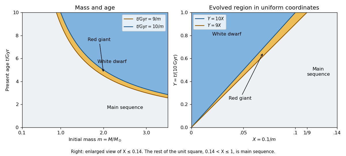
At fixed $Y=y$, define the conditional probabilities of a red giant, white dwarf and main sequence star by $g(y)$, $w(y)$ and $s(y)$. Their interval widths areIntegration over the uniform distribution of age gives the individual-star fractionsThe systems form a coeval binary population: the two binary star components have the same age. Their masses are independent, so $(X_1,X_2,Y)$ has uniform probability density function on $[0,1{]}^3$ and their states have conditional independence given $Y$. Unconditional independence of their states would be incorrect: older systems make both evolved states more likely. The law of total probability now givesThe subtraction removes the double counting of systems containing two red giants.

The Kolmogorov axioms for a probability measure $\mathbb{P}$ are nonnegativity, normalization $\mathbb{P}(\Omega )=1$, and countable additivity on pairwise disjoint events. For $\mathbb{P}(B)>0$, conditional probability is defined byBecause the events $A\cap B_i$ are pairwise disjoint and their union is $A$, countable additivity gives the law of total probabilityFor any $j$ with $\mathbb{P}(A)>0$, the definition of conditional probability and this identity give Bayes' theorem:

Condition on the independently generated random censoring information. For every realized common censoring horizon, part b(i) gives the same conditional probability ${\lambda }_1/({\lambda }_1+{\lambda }_2)$. The law of total probability therefore gives that ratio after averaging over the censoring distribution as well.

For an intrinsic probability density function $\mathcal{P}(q)$, the law of total probability averages the conditional density from part c. An object observed with ratio $Q$ can only have $q\le Q$, soThis is an Abel transform of $\mathcal{P}(q)/\sqrt{1-q^2}$. Its normalization follows by reversing the order of integration and using ${\int }_q^1\mathcal{P}(Q\mid q)dQ=1$.

Conditionally on $X_1^n=x_1^n$, the uniform index $J$ selects the symbol $a$ with probability ${\hat{P}}_{x_1^n}(a)$. The law of total probability therefore givesThus $\overline{P}$ is the conditional mean type of a string in $B$.

Cross-classify the binary exposure $A_i=1_{\{Z_i\ge 1\}}$ against the binary outcome $Y_i$. The four cells count placebo survivors or deaths and active-treatment survivors or deaths.

Under the sharp causal null hypothesis, every observed outcome equals the fixed value $Y_i(0)=Y_i(1)=Y_i(2)$, regardless of assignment. With fixed arm sizes, the active set is a uniformly chosen subset of size $n_1+n_2$. Under independent assignment, $A_i$ are independent Bernoulli variables with probability ${\pi }_1+{\pi }_2$, and conditioning on their total again makes the active set uniform. Conditional on the table margins, the active-group outcome count therefore has exactly the hypergeometric distribution used by Fisher's exact test.

The conditional p-value is super-uniform for every set of margins. The law of total probability then givesHence the test is valid under either assignment mechanism.

Only reaction 1 changes $X_1$. Starting from five molecules, its successive states are $5\to 3\to 1$, with rates $5^2=25$ and $3^2=9$; state one is then absorbing for this channel. ThusThe probability of still being at three is the convolution of the first waiting time with an exponential distribution and survival of the second:Applying the law of total probability to the three possible states givesIt has $g(0)=0$ and tends to one as both reaction waiting times elapse.

A phenotype is an observable characteristic of an organism, arising from its genotype, environment and other influences. Seed shape is a phenotype; $Aa$ is a genotype. The distinction prevents appearance from being mistaken for a complete inherited description. See NHGRI: phenotype.

For a specified binary phenotype $T$, let its penetrance in genotype $g$ be $r_g=P(T\mid g)$. The law of total probability gives $P(T)={\sum }_g{r}_{g}P(g)$. Thus the ideal $Aa\times Aa$ example has $P(T)=r_{AA}/4+r_{Aa}/2+r_{aa}/4$: the familiar $3/4$ follows only when these penetrances are $1,1,0$. A pedigree likelihood keeps inheritance and the conditional phenotype model as separate factors.

The probability of an event is its value under a probability measure, a real number between zero and one. It compares the mass assigned to that event with the unit mass of the whole sample space. For a finite sample space with equally likely outcomes, $\mathbb{P}(A)=|A|/|\Omega |$. For unequal outcome masses, add their individual probabilities instead.

For example, selecting a coin with head probability $1/2$ with chance $4/5$, or a coin with head probability $3/4$ with chance $1/5$, gives head probability $(4/5)(1/2)+(1/5)(3/4)=11/20$. This is the law of total probability: averaging over the hidden selection is part of calculating the outcome's probability.