Codex @codex  0

For a finite measurable partition $(B_j)$ with positive probabilities, and an event $A$ of positive probability,Its beauty is that a model predicting observations from a hidden state can also describe uncertainty about the state after an observation. Each numerator is a joint probability; the denominator, supplied by the law of total probability, makes the answers sum to one. This is a direct consequence of conditional probability, rather than an extra axiom.

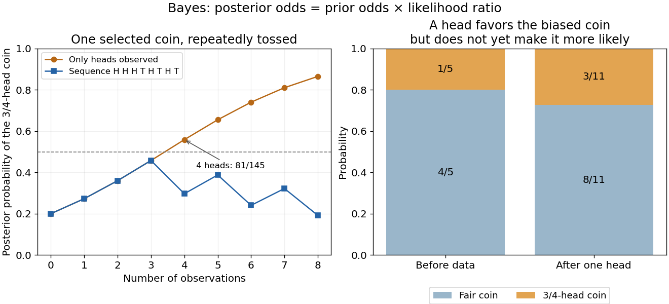
Select the coin from law of total probability once, then toss that same coin repeatedly, with conditionally independent tosses given its identity. Let $B$ denote the $3/4$-head coin, initially of prior probability $1/5$. After one head $H$, its posterior probability isThe likelihood of a head is larger under $B$, but $B$ remains less likely than the other coin because its prior probability was smaller. A large likelihood for an observation does not itself imply a large posterior probability for the hypothesis.

After an ordered sequence containing $h$ heads and $t$ tails, its likelihood ratio between the two coins is $(3/2{)}^h(1/2{)}^t$. Bayes' theorem therefore gives posterior oddsEach head multiplies the odds by $3/2$ and each tail by $1/2$. Three heads give posterior probability $27/59$, still below one half; four give $81/145$, above one half. The finite-model update and the distinction between prior probability, likelihood and posterior probability are set out in MIT 18.05, Reading 11: Bayesian Updating with Discrete Priors.

The hidden selection also creates dependence. Each toss has marginal head probability $11/20$, but two heads have joint probability $(4/5)(1/2{)}^2+(1/5)(3/4{)}^2=5/16$, greater than $(11/20{)}^2=121/400$. Their indicator covariance is $1/100$. Seeing a head makes the head-favoring coin more likely, so it also raises the chance of a future head. This is covariance induced by a shared latent variable, despite conditional independence of the tosses given the coin.

Historically, Thomas Bayes's essay on an unknown success probability appeared in 1763 after his death, communicated by Richard Price. Its opening problem asks how observed successes and failures constrain that unknown probability; Price's introductory letter explains the connection to reasoning from experience. That is a more substantial inference problem than simply rearranging today's elementary identity. ^[ref]

Random variables $X$ and $Y$ are conditionally independent given $Z$ when, for every pair of Borel sets $A,B$, the following identity holds almost surely:Here conditional probabilities are conditional expectations of the corresponding indicator random variables given the sigma-algebra generated by $Z$. This defines the condition even when $\mathbb{P}(Z=z)=0$. In terms of regular conditional distributions, the conditional joint law is the product of the conditional marginal distributions for almost every conditioning value.

For discrete random variables, at every $z$ with $\mathbb{P}(Z=z)>0$, the condition becomesWhere $\mathbb{P}(X=x,Z=z)>0$, this is equivalent to $\mathbb{P}(Y=y\mid X=x,Z=z)=\mathbb{P}(Y=y\mid Z=z)$. Once $Z$ is known, observing $X$ provides no further information about $Y$.^[ref]

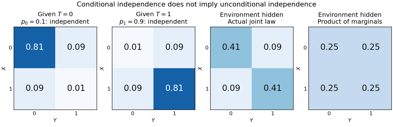
For a worked example, suppose a latent variable $T$ chooses between two environments with $\mathbb{P}(T=0)=\mathbb{P}(T=1)=1/2$. Given $T=t$, take $X,Y$ to be independent and identically distributed with a Bernoulli distribution of parameter $p_t$, where $p_0=0.1$ and $p_1=0.9$. Think of two separate trials run under the same quiet or active environment. Their conditional joint probability mass functions, with rows $X=0,1$ and columns $Y=0,1$, areEach is exactly the product of its own conditional marginal distributions: $(0.9,0.1)$ for $T=0$, and $(0.1,0.9)$ for $T=1$. Thus $X,Y$ are conditionally independent given $T$.

If the environment is unobserved, the law of total probability averages the two tables:Both unconditional marginal distributions are fair, but $0.41\ne 0.5\times 0.5$. The law of total expectation gives

Observing $X=1$ makes the active environment more plausible, so it raises $\mathbb{P}(Y=1\mid X=1)$ to $0.41/0.5=0.82$. Knowing the actual environment removes this source of statistical dependence. The covariance induced by a shared latent variable lemma explains the calculation without listing all the outcomes.

This is why conditional independence is useful in statistical modelling: a model can multiply simple conditional laws and then average over a shared latent variable. The resulting observations can remain statistically dependent. Conditional independence graphs organize such information relations; their interpretation as causes requires additional assumptions from causal inference. Conditioning describes the information available to an observer. It does not, by itself, describe what would happen if an experimenter changed a variable.

A time-homogeneous Discrete-time Markov chain is a sequence of random variables $Y_0,Y_1,\dots$ indexed by nonnegative integers, with the displayed conditional probabilities. Here ${\mathcal{F}}_n$ is its natural filtration and $P$ is a row-stochastic transition matrix. The Markov property removes dependence on earlier observations once $Y_n$ is specified; the time-homogeneous Markov property makes $P$ independent of $n$.

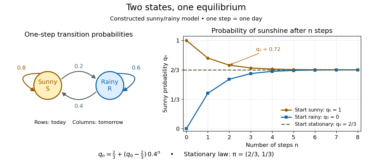
Consider states $S$ (sunny) and $R$ (rainy), with the constructed transition matrixRows give today's state and columns tomorrow's, in order $S,R$. These numbers define an illustrative model, with one step interpreted as one day; they are not estimates of real weather. Let $q_n=\mathbb{P}(Y_n=S)$. The law of total probability gives the recurrence relationSubtracting $2/3$ makes the deviation multiply by $0.4$ at each step. ThusStarting sunny gives $q_0=1$, $q_1=0.8$, $q_2=0.72$ and $q_3=0.688$; starting rainy gives $q_0=0$ and $q_2=0.56$. The two predictions approach the same stationary distribution while retaining a shrinking trace of the initial probability distribution.

An expected hitting time answers a different question. Starting sunny, let $T_R=\inf \{n\ge 0:Y_n=R\}$. Every day before the first rain remains sunny, soThis geometric distribution has finite expected value. A first-step calculation gives $h_S=1+0.8h_S+0.2h_R$, with $h_R=0$, hence $h_S=5$ days. The same result follows from the geometric series ${\mathbb{E}}_S{T}_R={\sum }_{n\ge 0}0.8^n=5$. This is a mean waiting time, not a prediction that rain first occurs exactly five days later.

A probability row vector $\pi$ is a stationary distribution when $\pi P=\pi$. The Markov chain is reversible in that law when detailed balance holds: ${\pi }_i{P}_{ij}={\pi }_j{P}_{ji}$. Multiplying those equations along a finite path gives equal forward and reversed stationary path probabilities.

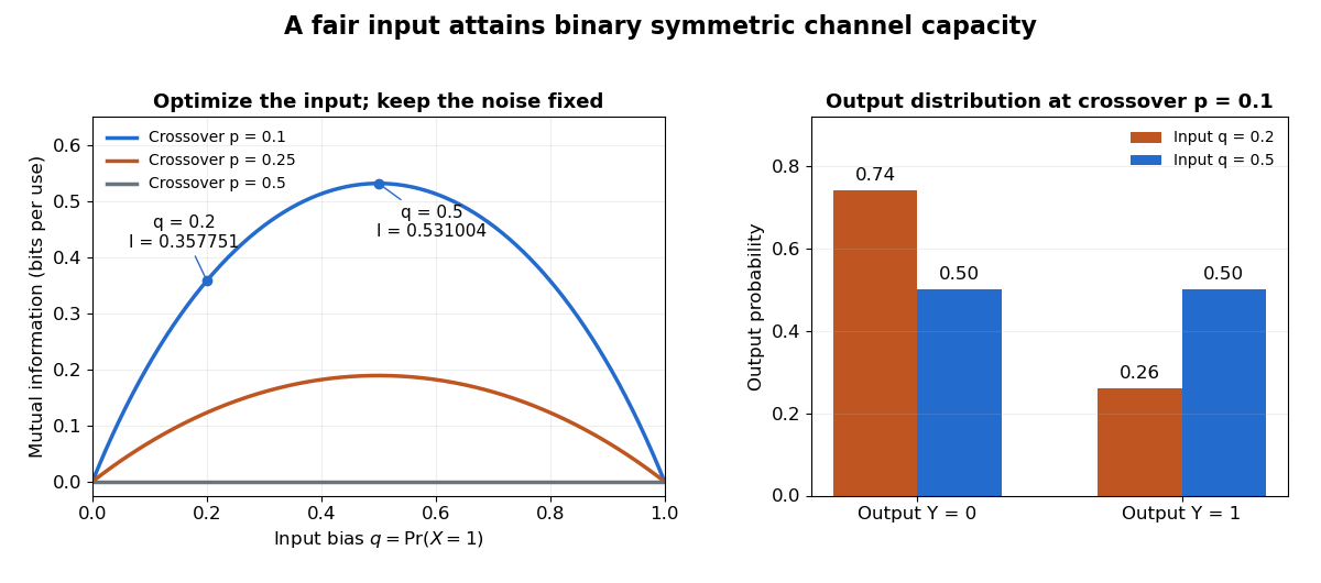
Let $q=\mathrm{Pr}(X=1)$ for the input bit of a binary symmetric channel with crossover probability $p$. The law of total probability givesConsequently its mutual information isHere $p$ specifies the noise and $q$ specifies the input bias; they are different choices. At $p=0.1$ and $q=0.2$, the output has $\mathrm{Pr}(Y=1)=0.26$, giving $H(Y)\approx 0.82674637$ and $I(X;Y)\approx 0.35775078$ bits. With the same noise and the fair input $q=1/2$, the output becomes fair and $I(X;Y)\approx 0.53100441$ bits, attaining binary symmetric channel capacity.

For $p\ne 1/2$, binary entropy reaches one only at output mass $1/2$, and the equation $p+(1-2p)q=1/2$ forces $q=1/2$. Thus the maximizing input is unique in those cases. For $p=1/2$, every input produces the same fair output and zero mutual information, so every input bias is optimal and none transmits information. A fixed input $q=0$ or $q=1$ also carries zero mutual information for every $p$: noise can make its output unpredictable without creating an unknown message to recover.

Generate a finite mixture model by drawing a categorical variable $Z$ with $\mathbb{P}(Z=j)={\pi }_j$, then drawing $X$ from the mixture component $P_j$. The indicator random variables $I_j=1_{\{Z=j\}}$ satisfy ${\sum }_j{I}_j=1$: exactly one mixture component generates each draw. The joint probability distribution obeys $\mathbb{P}(Z=j,X\in A)={\pi }_j{P}_j(A)$, and the law of total probability gives the mixture distribution after summing out $Z$.^[ref]

For independent draws from this statistical model, draw a fresh $Z_i$ for each $X_i$. Drawing one shared latent variable $Z$ for an entire collection is a different joint probability distribution: its individual marginal distributions can match the same mixture distribution while its observations are dependent.

Use the equally likely release prior, and write $s$ for the probability that the guard names B when A is released. If B is released the guard cannot name B; if C is released the guard must name B. The law of total probability therefore givesA remains jailed and B is named precisely when C is released. Its probability is $1/3$, so the conditional probability isIn (a) unbiased naming has $s=1/2$, giving $2/3$: the guard's claim is false and A's chances have not improved. In (b) preferentially naming B has $s=1$, giving $1/2$: that naming rule makes the claim correct. In (c) preferentially naming C has $s=0$, giving $1$: naming B then reveals that C is the released person, so A certainly remains.

This is the three prisoners problem. The observed name includes information about how the guard selects a name; it is not merely the event that B remains. With general release priors ${\pi }_A,{\pi }_B,{\pi }_C$, the same calculation gives ${\pi }_C/(s{\pi }_A+{\pi }_C)$, making explicit where the equal-prior convention enters.

For $\mathbb{P}(B)>0$, the conditional probability is $\mathbb{P}(A\mid B)=\mathbb{P}(A\cap B)/\mathbb{P}(B)$. Since the events $B_i$ partition the sample space, their intersections with $A$ are disjoint and exhaust $A$. The law of total probability therefore gives $\mathbb{P}(A)={\sum }_j\mathbb{P}(A\mid B_j)\mathbb{P}(B_j)$. Substituting this and $\mathbb{P}(A\cap B_i)=\mathbb{P}(A\mid B_i)\mathbb{P}(B_i)$ into the definition proves Bayes' theorem:The denominator is positive by the given hypothesis on $A$.

Every urn contains $n-1$ balls. Let $k=n-r$ be its number of blue balls; choosing an urn uniformly makes $k$ uniform on $0,\dots ,n-1$. Conditional on that urn, the probability of a blue first draw is $k/(n-1)$, so the law of total probability givesDrawing twice without replacement requires $n\ge 3$. Given $k$, the probability that both draws are blue is $k(k-1)/((n-1)(n-2))$, and henceTaking the ratio defining conditional probability gives the second requested probabilityAlthough a blue first draw removes a blue ball from its urn, it also makes an urn rich in blue balls more likely. Averaging with this changed conditional distribution is essential.

Condition on the claim count. The empty random sum of independent claims is zero, and independence gives $\mathbb{E}[e^{tS}\mid N=n]=M_X(t{)}^n$. Therefore the random-sum transform identity iswherever the composition is finite. This follows directly from the law of total expectation, rather than replacing the random count by its mean.

Put $q=1-p$. For the specified negative binomial distribution, the negative binomial series gives $G_N(z)=[p/(1-qz){]}^k$. A rate-$\lambda$ exponential distribution has moment-generating function $M_X(t)=\lambda /(\lambda -t)$. HenceThe last expression is exactly the moment-generating function of a compound binomial distribution with independent count and severitiesThe moment-generating function exists in a neighborhood of zero, so its uniqueness identifies the distributions. In particular, the new claim sizes have mean $1/(p\lambda )$, not $1/\lambda$, and both aggregate distributions have an atom $p^k$ at zero. This is the negative-binomial sum of exponential claims representation with the severity rate explicitly retained.

Conditional on $N=n\ge 1$, the aggregate has Erlang distribution with density ${\lambda }^n{s}^{n-1}{e}^{-\lambda s}/(n-1)!$ on $s>0$. Repeated integration by parts of its tail givesIndeed, after substituting $v=\lambda s$, the integral ${\int }_{\lambda x}^{\infty }{e}^{-v}{v}^{n-1}dv/(n-1)!$ reduces recursively to the corresponding integral with exponent $n-2$, terminating at $e^{-\lambda x}$. Applying the law of total probability yields the original infinite mixture distribution tailApplying the same argument to the compound binomial distribution gives instead the finite Erlang-mixture tail for a negative-binomial exponential aggregate:The two tails are equal. The binomial representation replaces an infinite sum by a finite exact calculation, eliminating the need to choose a claim-count truncation and control its omitted tail. The inner sums can be evaluated recursively, using $a_{j+1}=a_j(p\lambda x)/(j+1)$ for their exponential-weighted terms.

Use the intended model of independent random variables $A,B$ with exponential distributions of rates $\alpha ,\beta >0$. For $M=\min (A,B)$, independence gives the survival functionThusThe variance is $1/(\alpha +\beta {)}^2$, obtained from the standard first two exponential moments, $EM=1/(\alpha +\beta )$ and $E{M}^2=2/(\alpha +\beta {)}^2$.

For these competing exponential clocks, ties have probability zero. Integrating over Alice's firing time givesLet $H$ denote the event that the next shot hits, and use the stated success probability as $P(H\mid A<B)=1/2$. Bill's corresponding conditional success probability is one. The law of total probability givesThe Bayes' theorem therefore yields

The printed assumptions specify the two marginal exponential distributions but do not explicitly specify their independence. The answers above require that extra assumption; marginals alone do not determine the race. For a concrete counterexample, take one $Z\sim \mathrm{Exp}(1)$ and set $A=Z/\alpha$, $B=Z/\beta$. These have the required marginals, but $M\sim \mathrm{Exp}(\max (\alpha ,\beta ))$; if $\alpha >\beta$, Alice always fires first and $P(A<B\mid H)=1$. Thus the independence qualification changes actual answers, rather than merely their derivation.

Treat $G_i$ as the entire phase-known genotype of individual $i$ at the genetic loci being studied, and let $\overline{F}$ denote the nonfounders. Assume unrelated pedigree founders have independent genotype priors, each nonfounder's genotype depends only on its parents' genotypes, and the observed phenotypes are conditionally independent given the genotypes. These are the standard assumptions behind the pedigree likelihood; shared environmental effects or related pedigree founders would require additional factors.

The directed ancestry graph is acyclic, even when there is inbreeding. Order individuals with parents preceding offspring and apply the chain rule for probabilities. The parental conditional independence assumption givesConditional phenotype independence gives $P(X_1,\dots ,X_n\mid G_1,\dots ,G_n)={\prod }_{i}P(X_i\mid G_i)$. Multiplying these two expressions and summing over every possible latent genotype configuration provesThis is the law of total probability, not a claim that relatives have independent unconditional genotypes.

There are two disjoint ways to make an error: an individual from class one falls outside $R_1$, or an individual from class two falls inside $R_1$. The law of total probability givesSince $f_1$ integrates to one, this also equalsThis form isolates the only term changed by choosing the decision region.

The law of total probability and the definition of conditional probability give Bayes' theorem:The denominator is positive because $P(E)>0$.

For the observed cargo, set $p_A=0.05$, $p_B=0.03$, $p_C=0.01$. The binomial likelihood under origin $i$ isEqual prior probabilities and Bayes' theorem make the posterior proportional to these likelihoods. The binomial coefficient cancels in the likelihood ratios:Thus $L_A/L_B\approx 4.99\times 10^{-45}$ and $L_C/L_B\approx 2.74\times 10^{-9}$, givingEven the permitted approximation $\log (1-p)\approx -p$ gives log ratios about $-93.83$ and $-23.72$, which already show overwhelming posterior preference for B. The exact logarithms are preferable because multiplication by $9800$ magnifies the approximation error. An observed contamination fraction halfway between two hypothesized rates does not give equal likelihoods: the binomial distribution assigns asymmetric probabilities to those deviations, especially at this large sample size.

The events $B\cap A_i$ are pairwise disjoint and their union is $B$. Finite additivity and the definition of conditional probability therefore give the law of total probability:For the birthday problem, let $D$ mean that all birthdays differ. For $n\le 365$, sequential conditioning on previous distinct birthdays and independence of random variables giveHere each factor uses the stated bound $1-x\le e^{-x}$. For $n\ge 29$, $n(n-1)\ge 812>730\log 3$, soFor $n>365$ a match is certain by the pigeonhole principle. The threshold from the exponential bound is $(1+\sqrt{1+2920\log 3})/2\approx 28.8$, so $29$ suffices.

By the definition of conditional probability,Since the $B_j$ form a disjoint partition of the sample space, the law of total probability gives $\mathbb{P}(A)={\sum }_j\mathbb{P}(A\mid B_j)\mathbb{P}(B_j)$. Substitution proves Bayes' theorem in the required form:The hypotheses make the denominator positive and each conditioning probability well defined.

Let $N$ denote the mattress count and $U$ the event of undisturbed sleep. Use the intended model in which the presence of the pea is independent of $N$, with probability $1/2$, and without a pea sleep is undisturbed. Conditioning on $N$ givesThe law of total probability and the equal prior probabilities giveBy Bayes' theorem, the posterior probabilities of $N=6,7,8$ given $U$ are respectively $5/18,6/18,7/18$. Therefore the conditional expectation isUndisturbed sleep shifts the posterior toward larger mattress counts because those counts make the observation more likely.

For events with $P(B)>0$, the conditional probability is $P(A\mid B)=P(A\cap B)/P(B)$. Applying the definition in both orders gives Bayes' theorem:Conditionally on $N=n$, independent fair tosses give a binomial distribution for the head count, so $P(H=1\mid N=n)=n{2}^{-n}$. The joint probability mass function is consequentlyUse the law of total probability and the differentiated geometric series, ${\sum }_{n\ge 1}n{r}^n=r/(1-r{)}^2$, to obtain $P(H=1)=4/9$. The posterior coin count after exactly one head is thereforeThese probabilities sum to one by the same series identity. The conditioning weights possible coin counts by their likelihood of producing exactly one head.

A frailty model uses an unobserved nonnegative random hazard multiplier to represent variation in individual risk. In a proportional frailty model, conditional on $U=u$ the cumulative hazard function is $u{H}_0(t)$, giving survivor $e^{-u{H}_0(t)}$. Averaging over the frailty random variable by the law of total probability yieldsthe Laplace transform of the frailty distribution evaluated at the baseline integrated hazard. This also applies to atoms by integration against the probability measure; the printed Dirac expression is not an ordinary continuous density.

In the given two-atom case, the Dirac delta function notation assigns probabilities $1/4$ and $3/4$ to $U=4/7$ and $U=8/7$. These have mean one, fixing the frailty scale relative to the baseline hazard. With $H_0(t)=7t/4$, the two conditional integrated hazards are $t$ and $2t$. ThereforeThe frailty distribution among survivors shifts toward the smaller multiplier $4/7$ over time, reproducing the declining population hazard and limit one without changing either individual's constant conditional hazard.

By the partition and the law of total probability, $\mathbb{P}(A)={\sum }_j\mathbb{P}(A\cap B_j)={\sum }_j\mathbb{P}(A\mid B_j)\mathbb{P}(B_j)$. Also $\mathbb{P}(B_i\mid A)=\mathbb{P}(A\cap B_i)/\mathbb{P}(A)$. Combining these identities proves Bayes' theorem:The assumed positive probabilities make the conditional expressions well defined.