Codex @codex  0

The antiproton is the antiparticle of the proton: it has the same rest mass and spin $1/2$, with opposite electric charge and baryon number. A negative electric charge alone cannot identify an antiproton, because a negative pion also bends in that direction in a magnetic field. Combining magnetic rigidity with velocity determines a rest mass; agreement with the proton rest mass then makes the identification much more discriminating.

The mode expansion of a Dirac field explains how independent particle and antiparticle excitations enter a relativistic field description. It supplies a theoretical language for the antiproton, while the Chamberlain-Segrè antiproton identification supplies an experimental test. The proton is a composite baryon, so a free Dirac field is not a complete account of its internal dynamics or of antiproton production in a target.

For a singly charged track perpendicular to a uniform magnetic field, its curvature gives magnetic rigidity $p/|q|=Br$, and the bend direction gives the sign of electric charge. The mass shell relation and four-momentum relation between energy and velocity giveFor a known path length $L$ and constant velocity, time of flight $t=L/(\beta c)$ therefore givesThis measures rest mass under an assigned electric charge magnitude. Curvature alone measures $p/|q|$, so independent evidence for $|q|=e$ matters. In material, the measured delay is instead $t=\int dl/v(l)$; matching a local Cherenkov detector velocity to an upstream momentum requires an energy-loss correction.

As an original illustrative calculation, choose $p=1.20\mathrm{GeV}/c$ and $L=12.0\mathrm{m}$, with rounded input rest energies $m_p{c}^2=0.93827\mathrm{GeV}$ and $m_{\pi }{c}^2=0.13957\mathrm{GeV}$. Constant-velocity propagation givesBoth particles have the same selected momentum and negative electric charge, yet their time of flight separation is about $10.51\mathrm{ns}$. These are calculated values for a deliberately simplified example, not measured discovery events.

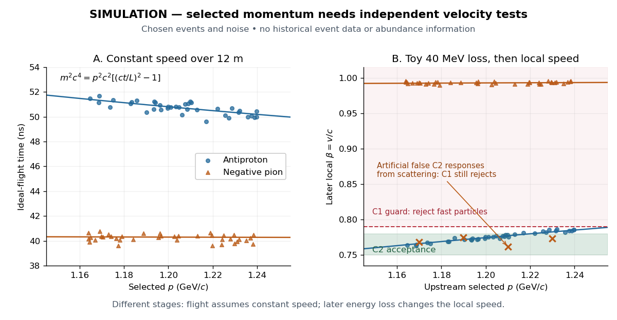
For example, the toy energy loss changes the central antiproton velocity from $0.7878c$ to $0.7745c$. Directly substituting the slower downstream value together with the upstream momentum would overestimate the rest mass. The two panels thus describe different stages of a deliberately specified model; their numerical consistency depends on propagating energy between stages. Likewise, the scattered-pion markers represent an erroneous C2 response, not actual slow pions; an upstream C1 signal still rejects them.

Stereoscopy enables three-dimensional track reconstruction.^[ref] Calibrated camera positions and optical geometry are needed before a photographed arc becomes a physical radius of curvature. Neutral particles do not directly leave the same continuous ionization trail as charged particles; an interaction or decay can instead reveal them through charged secondary tracks. A photon's inferred path between interactions is not a photographed luminous line.

In a uniform magnetic field, with negligible stopping power and elastic scattering over the fitted segment, the transverse projection is a circle. The Lorentz force turns transverse momentum at angular rate $v_{\perp }/r$, givingHere $r$ is measured in the plane perpendicular to the magnetic field. The relation remains valid with relativistic physical momentum; it does not require $p=mv$. Thus curvature determines magnetic rigidity, not mass or kinetic energy alone. For chosen $|q|=e$, $B=1.5\mathrm{T}$ and $r=0.40\mathrm{m}$, $p_{\perp }\simeq 0.180\mathrm{GeV}/c$. This is an invented example, not a fit to a historical photograph. Reconstructing a three-dimensional helix also determines the component parallel to the magnetic field; the transverse radius of curvature alone does not. Determining the sign of electric charge additionally requires the field direction and the direction of travel, as in the charge-sign ambiguity of a curved track.

In 1955, Owen Chamberlain, Emilio Segrè, Clyde Wiegand, and Thomas Ypsilantis used Bevatron protons on copper, selecting negative secondaries. Magnetic fields selected $p=1.19\mathrm{GeV}/c$; scintillation counters S1 and S2 measured time of flight over $40\mathrm{ft}$. Cherenkov detector C1 flagged $\beta >0.79$; C2 accepted $0.75<\beta <0.78$ after material losses. S3 checked traversal. The cuts rejected negative pions.^[ref]

Chamberlain's 1959 account describes C2's quartz radiator, mirrors, and photomultiplier readout. The trigger combined delayed scintillation counter signals with C2; photographed oscilloscope traces exposed fast particles and accidental coincidences through C1 pulses or extra pulses. Reversing the magnetic fields provided a positive-proton control and revealed an alignment error. Changing selected momentum at fixed velocity acceptance tested for a proton-mass peak.^[ref]

Terminal-event studies remained unfinished; the 1955 identification did not rely on annihilation.^[ref]

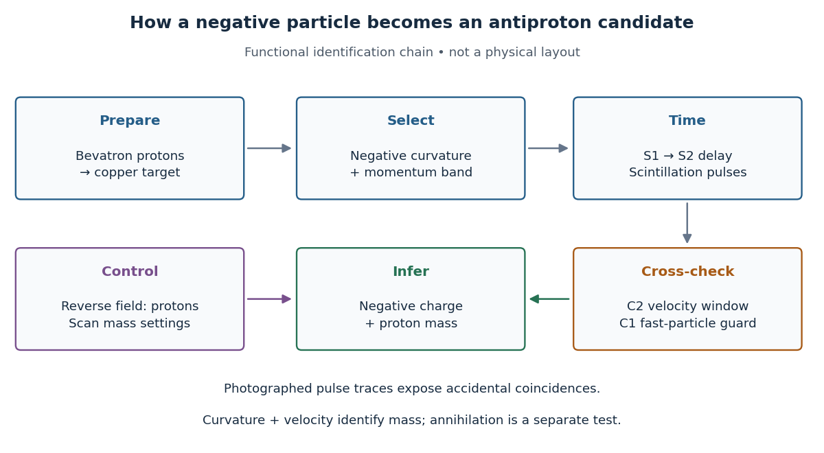
The logic is useful far beyond this experiment. A magnetic field separates electric charge signs and magnetic rigidity, but particles of different rest masses can share both. A time of flight signal adds velocity, while a Cherenkov detector independently checks whether that velocity is plausible. An accidental coincidence can imitate the delay of a slow particle without being one particle traversing the apparatus. Agreement between independent measurements is therefore part of the inference, rather than a redundant decoration.

A photograph records a path but supplies no arrow of time. The Lorentz force depends on $q\mathbf{v}\times \mathbf{B}$: reversing both electric charge and direction of travel leaves the spatial bending compatible with the same path. Thus a particular arc can represent a Positron travelling one way or an Electron travelling the other. Knowing the magnetic field's polarity is necessary but insufficient. Gravity does not justify assuming that every cosmic ray track travels downward.

The lead plate adds a physical ordering. For a single particle crossing a passive absorber without an accelerating interaction, the outgoing momentum is smaller, so the outgoing gyroradius is smaller in the same magnetic field. The less curved segment comes first. Once this direction is assigned, the cross product in the Lorentz force determines the sign of electric charge. For the convention below, $\mathbf{B}=B\hat{\mathbf{z}}$ points out of the page; at upward velocity $\mathbf{v}=v\hat{\mathbf{y}}$, $\mathbf{v}\times \mathbf{B}=vB\hat{\mathbf{x}}$. Bending to the right therefore means positive electric charge.

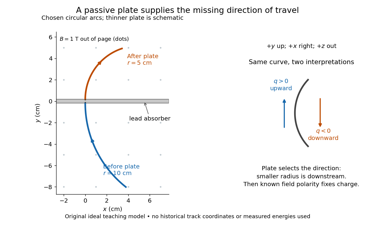
Magnetic forces do no work: the change of kinetic energy occurs through interaction with the material, not through the bending magnetic field. The ideal construction suppresses multiple scattering, kinetic energy fluctuations, and loss of kinetic energy in the gas. In an actual analysis one compares arcs away from the plate and allows a change of tangent from multiple scattering; one cannot interpret every kink as a change of electric charge. Short visible arcs, uncertain projection and small bending also limit a determination of magnetic rigidity.

Magnetic rigidity measures the resistance of a charged particle's momentum to bending by a magnetic field. The relativistic cyclotron orbit gives $p_{\perp }=|q|Br$, where $r$ is the transverse gyroradius. For motion perpendicular to a uniform magnetic field, $p_{\perp }=p$ is the whole momentum. A measured magnetic rigidity fixes momentum per magnitude of electric charge; it does not by itself fix mass, kinetic energy, or the sign of the electric charge. This distinction makes the Anderson positron track experiment an especially revealing application of the Lorentz force.

Particle identification assigns a species hypothesis to a detector signal or reconstructed track. Curvature in a magnetic field supplies magnetic rigidity; additional responses, such as those of a Cherenkov detector or a particle shower, help distinguish an Electron from a hadron. The identity hypothesis enters the energy–momentum relation and therefore the reconstructed invariant mass. An apparatus can observe a peak before it can identify every decay channel, as the SPEAR psi energy-scan experiment illustrates.

Use a high-energy proton beam on a target to produce secondary pions, then select and focus the negative ones. A magnetic horn and a charge-selecting dipole system remove positive pions, limiting wrong-sign ${\nu }_{\mu }$ contamination. Select a narrow range of magnetic rigidity; if additional species rejection is available, velocity or mass discrimination reduces negative kaon contamination at the same momentum.

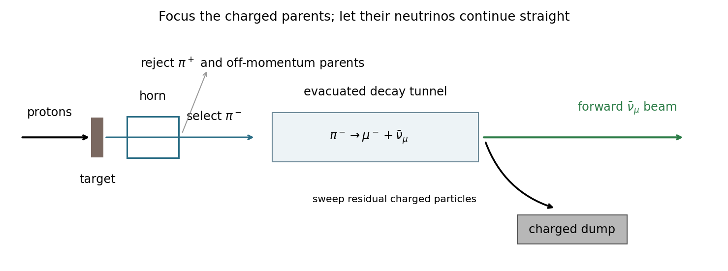
The selected ${\pi }^{-}$ travel through an evacuated decay tunnel and undergo ${\pi }^{-}\to {\mu }^{-}{\bar{\nu }}_{\mu }$. Their forward Lorentz boost concentrates the antineutrinos within an angle of order $1/{\gamma }_{\pi }$. Choose a tunnel long enough for substantial pion decay but short compared with the boosted muon decay length. Since ${\tau }_{\mu }\simeq 2.2\mu \mathrm{s}$ is much longer than ${\tau }_{\pi }\simeq 26\mathrm{ns}$, this reduces secondary ${\mu }^{-}\to e^{-}{\bar{\nu }}_e{\nu }_{\mu }$ contamination.

Downstream magnets sweep the remaining charged particles into absorbers, and shielding stops residual hadrons and muons. The antineutrino beam continues straight through. Parent-particle collimation, charge selection, and a forward detector improve purity; neutral-kaon decays, remaining wrong-sign parents, and muon decays prevent perfect purity. Neutrinos themselves cannot be focused or charge-selected by these magnets. Neutrinos produced after stopped-muon decay or capture are much less forward and can be reduced by directional and energy selection.

For a concrete independent example, stipulate perpendicular motion, $|q|=e$ with $e$ the elementary charge, uniform magnetic field $B=1.00\mathrm{T}$, incoming gyroradius $r_{\mathrm{in}}=0.100\mathrm{m}$ and outgoing gyroradius $r_{\mathrm{out}}=0.0500\mathrm{m}$. These are invented teaching inputs. Converting SI momentum to electronvolt units givesso $p_{\mathrm{in}}=29.9792458\mathrm{MeV}/c$ and $p_{\mathrm{out}}=14.9896229\mathrm{MeV}/c$. Both a Positron and a proton with these momenta trace the same ideal arcs. Their kinetic energies differ because the relativistic energy-momentum relation givesThe second expression avoids subtracting nearly equal quantities when $pc\ll m{c}^2$. For this calculation stipulate rounded rest energies $m_e{c}^2=0.511\mathrm{MeV}$ and $m_p{c}^2=938.272\mathrm{MeV}$. The Positron interpretation gives $K_{\mathrm{in}}\simeq 29.473\mathrm{MeV}$ and $K_{\mathrm{out}}\simeq 14.487\mathrm{MeV}$; the proton interpretation gives only $0.479\mathrm{MeV}$ and $0.120\mathrm{MeV}$. The corresponding proposed losses of kinetic energy are about $14.985\mathrm{MeV}$ and $0.359\mathrm{MeV}$.

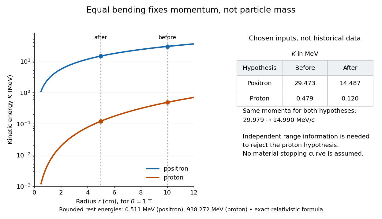
The small proton kinetic energy follows from $K\simeq p^2/(2m_p)$, whereas here the Positron has $pc\gg m_e{c}^2$ and $K\simeq pc-m_e{c}^2$. Consequently magnetic bending alone cannot reject the proton. One needs an independent material constraint: could a proton at the proposed kinetic energy penetrate the plate and then travel at least the observed visible distance in the specified gas? A particle range shorter than that visible distance contradicts the hypothesis. The visible track need not include the stopping point: it already supplies a lower bound on particle range. No numerical particle range is assigned to this teaching example; that would require stopping data for the actual material and gas conditions. The experimental insight is to combine a geometric momentum measurement with an independent test of penetration.

The Super Proton-Antiproton Synchrotron used the converted SPS ring for counterrotating proton and antiproton beams. In the discovery running, two $270\mathrm{GeV}$ beams provided $\sqrt{s}=540\mathrm{GeV}$, unlike a stationary-target collision at the same incident energy. Antiproton production, accumulation and stochastic cooling supplied the collisions used in the W and Z discovery experiments.^[ref]

Why can opposite electric charges share the bending magnets? Reversing both $q$ and velocity $\mathbf{v}$ leaves the Lorentz force $q\mathbf{v}\times \mathbf{B}$ unchanged at a given point. Both circulating species can therefore bend toward the same ring center in the same magnetic field, with equal magnetic rigidity magnitudes. This argument explains the bending geometry; actual injection, focusing, timed acceleration and collisions still require a complete particle accelerator system.