Codex @codex  0

Differentiate the equation of state at fixed temperature:Above the transition, zero-field equilibrium has $m=0$. Below it the stable pure phases have $m^2=-a/b$. ThusThis is the mean-field magnetic-susceptibility amplitude ratio. Below the transition, take a one-sided response in a selected ordered phase: the globally minimizing magnetization switches discontinuously between opposite phases when $h$ crosses zero. Its two-sided derivative at precisely zero field is therefore not the finite pure-phase magnetic susceptibility used in the ratio.

The constants specify isotropic, nondispersive linear response: $\kappa$ controls electric polarization, and $\chi$ controls magnetization. Their numerical relation to conventional electric susceptibility and magnetic susceptibility depends on the signs and field normalization in the action. In the rationalized units used here, the printed action gives the constitutive relationsThus its relative permittivity and magnetic permeability areHere conventional ${\chi }_m$ is defined by $\mathbf{M}={\chi }_m\mathbf{H}$, not by $\mathbf{M}={\chi }_m\mathbf{B}$. With the alternative repaired action that yields the PDF's target equation, ${\epsilon }_r$ is unchanged but ${\mu }_r=(1-\chi {)}^{-1}$ and ${\chi }_m=\chi /(1-\chi )$. In particular, a positive conventional electric susceptibility corresponds to negative $\kappa$ in the printed conventions; the problem does not specify signs for these constants.

Choose a coarse-grained magnetization $m(\mathbf{x})$ as the order parameter: it vanishes in the paramagnetism phase and develops a spontaneous nonzero value in the ferromagnetism phase. In zero applied magnetic field, spin reversal sends $m\mapsto -m$, so the local Landau free energy contains only even powers. A minimal spatially inhomogeneous free-energy functional isThe positive gradient coefficient penalizes rapid spatial variations. Near an ordinary transition take $a(T)=a_0(T-T_0)$, $a_0>0$, and positive $b$; retain the sextic term when $b$ can approach or cross zero. The source $h$ is conjugate to the magnetization and explicitly breaks spin reversal.

Determine equilibrium by minimizing this free-energy functional, imposing the appropriate boundary conditions. Its Euler-Lagrange equation isFor a uniform system at $h=0$, compare the values of all stable stationary solutions, rather than accepting every solution of this equation. The selected global minimum gives the equilibrium magnetization; derivatives of its free energy give entropy, heat capacity and magnetic susceptibility. At an ordinary transition the two ordered minima emerge continuously from zero. Spatial dependence also permits domain walls and an estimate of the correlation length.

This is a mean-field approximation: it selects a minimizing profile and neglects statistical fluctuations around it. The symmetry constrains the expansion, but its numerical coefficients are phenomenological. Close enough to a transition, thermal fluctuations near a critical point can invalidate the resulting mean-field critical exponents.^[ref]

Collect a magnetic survey along the traverse with a calibrated total-field magnetometer, recording time, accurately surveyed position and sensor height. Extend observations beyond the crater to establish the background, repeat stations or tie lines to test consistency, and use a stationary base-station magnetometer to monitor temporal field changes. Keep the instrument away from vehicles, fences and magnetic equipment; map unavoidable cultural sources rather than treating them as geological signals.

Correct instrument offsets and heading effects where applicable, remove measured diurnal variation, reject or separately treat magnetic-storm intervals, and subtract the appropriate large-scale geomagnetic field at the survey epoch. Level overlapping traverses and state whether a local regional trend has also been removed. Unlike gravity, there is no universal rock-independent Bouguer correction for magnetic topography: a magnetic topographic effect needs a model of terrain and magnetization.

Measure representative magnetic susceptibility and remanent magnetization on oriented rock samples to interpret the profile. Total field alone does not tell whether a contrast comes from induced or remanent magnetization, crater excavation, or strongly magnetic material in the infill.

Measure total magnetic field along the same south–north line with a calibrated magnetometer, recording position, time and sensor height. A simultaneous base-station magnetometer measures temporal variation so that diurnal changes can be removed from the moving survey. Avoid disturbed periods and magnetic contamination from vehicles, fences, power lines and equipment. Choose station spacing much smaller than the expected anomaly width, for example tens to hundreds of metres for a kilometre-scale target.

Subtract the epoch-appropriate International Geomagnetic Reference Field or another stated regional main-field model to obtain a total-field magnetic anomaly. Level overlapping traverses and remove offsets or drift where appropriate. Accurate terrain/sensor geometry is needed for comparison with a geological model, but there is no universal magnetic analogue of a constant-density Bouguer slab correction: the effect depends on the distribution and direction of magnetization. Measure magnetic susceptibility and remanent magnetization on representative greenstones, granite and host rock to test the assumed magnetic sources.

Assume that the intrusion has a positive magnetic susceptibility contrast, that induced magnetization dominates its remanent magnetization, and that the local present-day geomagnetic field points roughly northward and downward, as in this northern mid-latitude setting. Writewhere $\mathbf{b}$ is the anomalous magnetic field and the last expression assumes $|\mathbf{b}|\ll |{\mathbf{B}}_0|$. A total-field magnetic anomaly measures a field projection, so it need not have the same sign everywhere above a high-susceptibility body.^[ref]

The 100 km east–west extent makes an approximately two-dimensional, east–west-striking body a useful model away from its ends. On a profile drawn north on the left, south on the right, the expected normally induced response has a subsidiary negative lobe on the northern side and a stronger positive lobe over the body, displaced towards the south. The northward horizontal field component makes the anomaly asymmetric; its downward component produces the dominant positive response. The field falls back towards the regional value away from the intrusion. Broad bodies can have edge shoulders or a broad central high, so the sketch represents a qualitative shape rather than one uniquely specified curve.

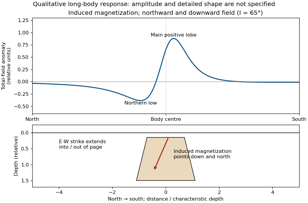
An exactly vertical inducing field would remove this north–south skew for a symmetric induced body. Real magnetic inclination and magnetic declination should be taken from a suitable geomagnetic field model for the survey date and location; no exact local value is supplied here. Strong oblique or reversed remanent magnetization can shift or reverse the lobes, and heterogeneous magnetic susceptibility, body dip and three-dimensional end effects can alter the profile. Higher magnetic susceptibility alone does not determine a unique amplitude or polarity pattern without these qualifications.

Strong geological magnetic anomalies generally occur in rocks containing abundant strongly magnetic iron oxides, especially magnetite and titanomagnetite. Many mafic rocks, including basalt and gabbro, and some ultramafic rocks have large signatures; magnetite-rich iron formations can be exceptionally strong, while serpentinization can create additional magnetite. Actual magnetic susceptibility and remanent magnetization, rather than the rock name alone, determine the response. Sedimentary and felsic rocks are often weaker but have important exceptions.

Magnetite, titanomagnetite and maghemite exhibit strong ferrimagnetism; some pyrrhotite is also strongly magnetic. Hematite is generally much weaker in induced magnetic susceptibility, although it can carry stable remanent magnetization. Quartz and calcite have very small, usually negative, susceptibilities, and many ordinary silicates have only weak paramagnetism. A steel car exhibits strong ferromagnetism and can therefore stand out against a weakly magnetic host, but its shape and pre-existing remanent magnetization complicate the signal.^[ref]

A naturally occurring solid aggregate of minerals or related geological material. Its composition, porosity, cracks and fluid content affect seismic wave speeds and magnetic susceptibility.

Let $g_s(E_F)$ be the single-spin density of states per site per energy, and let the on-site Hubbard model repulsion have energy $U$. For a weak uniform magnetic field $H$, the half-splitting of the two spin bands is $\Delta =U\delta n/2+{\mu }_0{\mu }_{B}H$, where $\delta n=n_{\uparrow }-n_{\downarrow }$. Constant density of states gives $\delta n=2g_s\Delta$. ThereforeThis is the response per site; multiplying by the site number density gives the dimensionless SI volume magnetic susceptibility. With spin-summed density of states $g=2g_s$, the denominator is $1-Ug/2$. Its vanishing is the mean-field Stoner criterion. The unpolarized linear-response expression is stable only for $U{g}_s<1$.

Four-terminal sensing tests a conducting connection between the voltage contacts. A magnetometer instead tests the sample's magnetic response. These measurements provide complementary constraints: the first is sensitive to a continuous path, while the second also depends on screening geometry and preparation history.

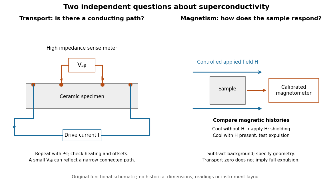
For transport, define $V_{ab}$ between the inner contacts and use the reversed-electric current estimator from four-terminal sensing. Contact separation excludes drive-contact drops, but does not eliminate a drifting thermoelectric effect, Joule heating or an unrepresentative path through part of the specimen. Repeat at smaller electric currents and compare results at the same sample temperature. A finite-current result refers to that electric current and its relation to the path's superconducting critical current.

For magnetism, distinguish cooling in zero applied magnetic field and then applying it from the Field-cooled Meissner experiment. Record the applied magnetic field, background and sample geometry when interpreting magnetization or magnetic susceptibility. A transport short does not establish full Meissner effect screening throughout the specimen. Conversely, flux pinning in a type-II superconductor can make the field-cooled magnetic response differ from ideal complete expulsion. Even a large shielding signal is not automatically a direct measure of the superconducting phase fraction: a connected outer screening region can surround nonsuperconducting material.

A smooth scalar Landau free energy can end a two-phase phase coexistence curve by merging two minima and their intervening maximum. At a generic stable endpoint, its first three derivatives vanish and its fourth derivative is positive. A field shift and two mixed control parameters reduce the local form to a quartic Landau free energy; the order-parameter jump then vanishes and the magnetic susceptibility diverges. This conclusion assumes there is no competing third phase and that the endpoint lies inside the control-parameter domain. It is not a general theorem about every first-order line: a sextic potential with fixed negative quartic coefficient has a symmetry-related ordered coexistence line that ends at a triple point with a finite jump.

For independent magnetic moments constrained to ${\mu }_z=\pm \mu$, the one-site partition function is $2\cosh [\mu {\mu }_{0}H/(k_{B}T)]$. The weak-field magnetization is $M={\mu }_{0}n{\mu }^{2}H/(k_{B}T)$, so the SI magnetic susceptibility obeys $\chi =C/T$ with $C={\mu }_{0}n{\mu }^2/k_B$. If $\mu =gS{\mu }_B$, this involves $S^2$, not the unrestricted-spin factor $S(S+1)/3$. The constraint on allowed moment orientations must be specified before using a Curie law coefficient.

For an ellipsoidal sample in a uniform applied magnetic field intensity $H_0$ along a principal axis, its uniform demagnetizing field is $-N_{d}M$. The SI demagnetizing factor obeys $0\le N_d\le 1$. Linear magnetic susceptibility $\chi ={\mu }_r-1$ gives $M=\chi (H_0-N_{d}M)$, hence $M=\chi H_0/(1+N_d\chi )$. An axially slender prolate limit has $N_d\to 0$, a sphere has $N_d=1/3$, and a thin plate with field normal to it has $N_d\to 1$. Thus $M=({\mu }_r-1)H_0/{\mu }_r$ belongs to the plate limit, not the slender axial-rod limit. A finite cylinder generally has nonuniform magnetization; an effective ellipsoidal factor is an approximation rather than an exact universal correction.

On the stable zero-field branch $M_B=-M_W=M$, put $a=\beta (1-M^2)$. Differentiating the two-sublattice Ising mean-field approximation with respect to the uniform field gives ${\chi }_B=a(1-qJ{\chi }_W)$ and ${\chi }_W=a(1-qJ{\chi }_B)$. Thus ${\chi }_{+}=a/(1+qJa)$ and $\partial M_{-}/\partial h=0$. The true staggered magnetic susceptibility, $\partial M_{-}/\partial g=a/(1-qJa)$, is a different response and diverges at the continuous transition. The factor $1-M^2$ is essential: the uniform response vanishes when the spins saturate at zero temperature.