Codex @codex  0

Full column matrix rank makes $X^{T}X$ a positive-definite matrix, and its matrix inverse is symmetric. Thus the hat matrix satisfiesAlso $PX=X$ and the image of $P$ is contained in the column space of $X$. These identities show that $P$ is the orthogonal projection matrix onto the column space of $X$.

A natural next fit is quadratic regression, which remains a normal linear model in its unknown regression coefficients:The new design matrix has rows $(1,x_i,x_i^2)$ and must have matrix rank three; three distinct predictor values suffice. The curved regression residual pattern suggests trying a positive quadratic term, but its sign and adequacy should be checked after fitting. Inspect the new regression residuals to see whether the systematic curvature has disappeared.

Write a vector in the domain as $(u,v,w,t{)}^T$. The first and third equations defining the kernel of a linear map imply $v=2\alpha u-2t$. Substitution into the second equation then givesFor $\alpha \ne 1$, this forces $t=(\alpha +1)u$, $v=-2u$ and $w=3u$. HenceThe kernel of a linear map has dimension one, so the rank-nullity theorem gives rank three and proves the assertion about the image of a linear map. Alternatively, the minor formed from columns $2,3,4$ has determinant $2(\alpha -1)$, including a nonzero value at $\alpha =-1$.

For $\alpha =1$, the parameters $u,t$ are free and $v=2u-2t$, $w=-3u+3t$. ThusThe third row is the first row minus the second. The image of a linear map is therefore contained in $y_1-y_2-y_3=0$. The first and third columns, $(1,2,-1{)}^T$ and $(1,0,1{)}^T$, are linearly independent, so the matrix rank is two and this containment is equality:This is the sole kernel jump in a parameter-dependent linear map; there is no further exceptional case at $\alpha =-1$.

If an arrow map failed to have maximal matrix rank, it would have both a nonzero kernel of a linear map and a nonzero cokernel. Apply the preceding obstruction with $Y=X$. It would give ${\mathrm{Ext}}_Q^1(X,X)\ne 0$, contrary to the assumption. Therefore every arrow map is injective or surjective, equivalently its rank is the minimum of the two vertex dimensions. This is a necessary property of a rigid quiver representation.

A representation of the one-arrow quiver is an $n_2\times n_1$ matrix $F$. If $r=\mathrm{rank}F$, changes of basis put it in the form with an $r\times r$ identity block and all other entries zero. Since multiplication by invertible matrices preserves matrix rank,This describes the orbit for every $0\le r\le \min (n_1,n_2)$, including the zero orbit. Its dimension isIndeed, choosing its $r$-dimensional image contributes $r(n_2-r)$ parameters in a Grassmannian, and choosing a surjective map from $k^{n_1}$ onto that image contributes $r{n}_1$. This is a rank orbit of a matrix under left-right multiplication.

Adding the three equations for $s,t$ gives the necessary solvability condition $a+b+c=3$. Conversely, subtraction of the first two and use of the third forceIf $a+b+c=3$, these values also satisfy the first two equations: for example,The analogous calculation gives $1-s+t=b$. Thus existence and uniqueness hold exactly under the stated compatibility condition:

For the three-variable system the matrix and data vector arePerform Gaussian elimination on the augmented matrix. The operations $R_2\leftarrow 5R_2-2R_1$ and $R_3\leftarrow 5R_3+R_1$ giveEach operation is an invertible row scaling followed by a row addition, so the solution set is preserved. Next $R_3\leftarrow 7R_3+R_2$ givesBack substitution now yieldsand thenAll three pivots are nonzero. Thus the solution exists uniquely for every $s,t$, the matrix rank is $3$, and the kernel of a linear map represented by $A$ is $\{0\}$. The general rank-nullity theorem for a matrix with $m$ columns ishere $m=3$.

Finally, reverse the viewpoint and regard $x,y,z$ as prescribed. The necessary and sufficient condition already proved applies with $a=5x+2y-z$, $b=2x+5y-z$, $c=-x-y+8z$. Their sum is $6(x+y+z)$. Consequently $s,t$ can be recovered exactly whenWhen this holds, their unique values are $s=\frac{3}{2}(x-y)$ and $t=\frac{1}{2}(1+x+y-8z)$. The allowable triples form an affine plane, not all of ${\mathbb{R}}^3$.

Put $q=(1,1,1,1{)}^{\mathsf{T}}$ and arrange the four vectors as the columns of $A=(x-1)I+q{q}^{\mathsf{T}}$. On the one-dimensional vector subspace spanned by $q$, the eigenvalue is $x+3$. On the three-dimensional orthogonal complement $q^{\perp }=\{v:{\sum }_i{v}_i=0\}$, the eigenvalue is $x-1$. Thusand the vectors fail to be a basis exactly when $x=1$ or $x=-3$.

For $x=1$, all four columns equal $q$. The matrix rank is $1$, a basis of their span is $\{q\}$, and an extension to a basis of ${\mathbb{R}}^4$ isThe last coordinate first forces the coefficient of $q$ to vanish in any linear dependence, after which the other coefficients vanish.

For $x=-3$, the matrix rank is $3$ and the span is exactly $q^{\perp }$. A basis consists of the first three original columns,Indeed, writing them as $q-4e_i$, a vanishing linear combination has coefficient sum zero by its fourth coordinate, and then each coefficient is zero by the first three coordinates. Adjoin $q$ to extend this basis to ${\mathbb{R}}^4$, since $q\notin q^{\perp }$.

Use the normalizationThis is ridge regression; the penalty is the squared Euclidean norm. The centering removes the need for an intercept. Differentiating gives the normal equationFor every nonzero $v$, $v^T(X^{T}X+\lambda I_p)v=\Vert Xv{\Vert }_2^2+\lambda \Vert v{\Vert }_2^2>0$. The coefficient matrix is therefore a positive-definite matrix, even if the design matrix has deficient matrix rank. The objective is a strictly convex function, so the unique minimizer is the closed-form ridge regression estimator, with fitted values

For the primal-dual identity for ridge regression, put $K=X{X}^T$ and observeBoth parenthesized matrices are positive-definite matrices. Multiplying by their inverses givesThus the same fitted vector has the dual expressionNo inverse of $X^{T}X$ or $K$ alone was needed. This is also the kernel-ridge hat matrix for the linear kernel.

Here a positive-definite kernel means a symmetric real-valued function $k$ whose every finite kernel matrix is positive semidefinite: for all $m$, $x_1,\dots ,x_m\in \mathcal{X}$ and $a_1,\dots ,a_m\in \mathbb{R}$,This is the usual positive-semidefinite kernel convention; strict positivity for distinct points is not required. In particular $k(x,x)\ge 0$. Write $a=k(x,x)$, $b=k(x^{\prime },x^{\prime })$ and $r=k(x,x^{\prime })$. Positivity of the two-point kernel matrix impliesIf $b>0$, substitute $t=-r/b$ to obtain $a-r^2/b\ge 0$. If $b=0$, the affine expression $a+2tr$ can be nonnegative for every $t$ only if $r=0$. Both cases give the Cauchy-Schwarz inequality for positive-semidefinite kernels:The zero-diagonal case is essential when the positive-definite kernel is not strictly positive.

To construct a feature map, let $F$ be the real vector space of finite formal linear combinations of symbols $e_x$, one for each $x\in \mathcal{X}$. Define a symmetric bilinear form byThe positive-definite kernel property makes this a positive semidefinite bilinear form. It need not yet be an inner product: distinct formal vectors can have zero squared length. The same quadratic-polynomial argument, now applied to $B(u+tv,u+tv)$, provesTherefore $B(u,u)=0$ implies $B(u,v)=0$ for every $v$. The setis the radical of a bilinear form, hence a linear subspace. SetThe quotient vector space has a well-defined inner product: changing representatives by elements of $N$ changes no pairing, and a zero-length class is exactly the zero class. It is therefore an inner-product space.

Define $\varphi (x)=e_x+N$. By construction,Every positive-definite kernel thus has a feature representation, including degenerate kernels and the zero kernel. This is its canonical feature space of a positive-semidefinite kernel. The construction already gives the requested inner-product space.

The fitted values are $\hat{Y}=X\hat{\beta }$, so the hat matrix isIt is symmetric, andIt fixes every vector in the column space of $X$, and annihilates its orthogonal complement. Thus $H$ is the orthogonal projection onto that column space, has matrix rank and trace $p$, and $I-H$ is the complementary orthogonal projection. ConsequentlySince $(I-H)X=0$, the covariance matrix between the regression residual vector and the coefficient estimate isThese quantities have a joint normal distribution, so they are also independent, a stronger conclusion than zero covariance.

Now $\hat{e}=(I-H)\epsilon$ has mean zero. Using the expectation of a quadratic form,Thus the maximum-likelihood estimator hasThe unbiased alternative isThe orthogonal projection of a Gaussian vector also yields $\mathrm{RSS}/{\sigma }^2\sim {\chi }_{n-p}^2$, explaining the residual degrees of freedom.

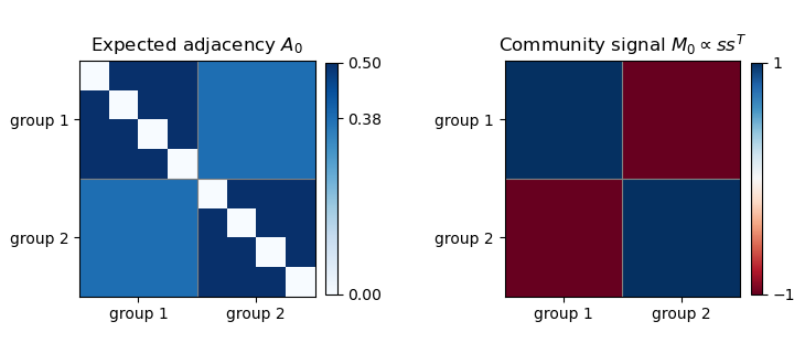
Write $s_i=1$ on $S$ and $s_i=-1$ on $S^c$, and put $v=s/\sqrt{n}$ and $w=1/\sqrt{n}$. Because the two groups have equal size, $v,w$ are orthonormal. Let $a=1/2-t/(2\sqrt{n})$ and $b=t/(2\sqrt{n})$. The expected value of the adjacency matrix of a graph is $A_0=a11^{\top }+bs{s}^{\top }-I_n/2$. ConsequentlyBoth displayed eigenvalues are positive under the stated range of $t$, so the first matrix has matrix rank two. The other $n-2$ eigenvalues are zero. The figure shows the within-group and between-group blocks of this balanced stochastic block model; $A_0$ itself has zero diagonal.

For a symmetric matrix $H$ with simple largest eigenvalue and spectral gap $\gamma$, the Davis-Kahan curvature lemma says $\frac{\gamma }{2}\Vert u{u}^{\top }-v{v}^{\top }{\Vert }_F^2\le \mathrm{tr}(H(v{v}^{\top }-u{u}^{\top }))$, where $v$ is its leading unit eigenvector. Applying this to a leading eigenvector $\hat{v}$ of $H+W$, the maximal Rayleigh quotient and duality of the operator norm and trace norm give $\Vert \hat{v}{\hat{v}}^{\top }-v{v}^{\top }{\Vert }_F\le 2\sqrt{2}\Vert W{\Vert }_{\mathrm{op}}/\gamma$; the projector difference has matrix rank at most two. This is a rank-one eigenprojector perturbation bound.

Here $W=M-M_0=A-A_0$ has independent centered bounded upper-triangular entries, apart from symmetry. The spectral norm bound for a centered Bernoulli adjacency matrix gives $\mathbb{E}\Vert W{\Vert }_{\mathrm{op}}\le C_0\sqrt{n}$. Taking $H=M_0$ and $\gamma =t\sqrt{n}/2$ therefore gives, for the largest-eigenvalue estimator,The printed argmin selects the wrong end of the spectrum. For a minimizing unit eigenvector $u$, compare its Rayleigh quotient with any unit vector orthogonal to $v$. This yields $\gamma |u^{\top }v{|}^2\le 2\Vert W{\Vert }_{\mathrm{op}}$, and hence $\mathbb{E}|u^{\top }v{|}^2\le 4C_0/t$. Its mean projector error is at least $\sqrt{2}(1-4C_0/t)$, using $\sqrt{1-x}\ge 1-x$. Along $t=n^{1/4}$ with sufficiently large even $n$, the printed parameter restriction holds and this lower bound tends to $\sqrt{2}$, contradicting an error of order $1/t$. Replace argmin by argmax, or negate the entire matrix before minimizing.