Codex @codex  0

A suitable Poincare disc automorphism is the Möbius transformationIt sends $a$ to zero and has inverse $(w+a)/(1+\overline{a}w)$. To verify the isometry directly, note thatThese identities show both that $f$ maps the unit disc onto itself and that $2|df|/(1-|f{|}^2)=2|dz|/(1-|z{|}^2)$, preserving the Riemannian metric.

Cross-ratio conventions differ by permutations. Use the following ordering, which gives the signs requested in part (c):Values involving infinity are defined by limits. This is the cross-ratio with second point mapped to zero: the Möbius transformationsends $z_1,z_2,z_4$ to $1,0,\infty$ and sends $z_3$ to $r$.

For $M(z)=(az+b)/(cz+d)$, $ad-bc\ne 0$, the identityshows that all factors cancel in the cross-ratio. This proves Möbius invariance of the cross-ratio, with the cases involving infinity following by limits. Algebraic subtraction also givesThe latter expression is another common ordering for the cross-ratio; keeping the convention explicit prevents an incorrect reciprocal or sign.

With $T$ from part (a), the first, second and fourth points map to $1,0,\infty$. The inverse image of the extended real line under a Möbius transformation is a generalized circle, meaning a circle or a line together with infinity. Thus, if $r=T(z_3)$ is real, all four original points lie on that generalized circle.

Conversely, if the four points lie on one generalized circle, its image under $T$ is another generalized circle containing $0,1,\infty$. A generalized circle containing infinity is a line, and the line through zero and one is the real line. Therefore $T(z_3)=r$ is real. Hence the cross-ratio is real exactly when the four points are concyclic or collinear.

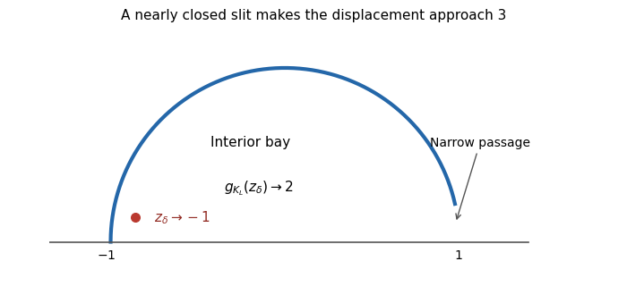
A nearly closed semicircular slit makes the constant sharp. PutThis is the unit-circle arc attached at $-1$ and ending just short of $1$. Its complement is a simply connected domain. There remains a narrow passage near $1$ connecting the interior bay to infinity. Thus $K_L$ is a compact H-hull inside the closed unit disc.

For an explicit check, let $S=\sqrt{1+L^2}$ and let $q_L(z)=\sqrt{m(z{)}^2+L^2}$ denote the mapping-out function of a vertical slit applied to $m(z)$, with the branch asymptotic to its argument in the slit half-plane. Its normalized map isThe final Möbius transformation takes the image of the original infinity to infinity and gives hydrodynamic normalization at infinity. For a fixed $z$ in the open unit half-disc, $\mathrm{Re}m(z)>0$, so $q_L(z)\sim L$ and $g_{K_L}(z)\to 2$ as $L\to \infty$. Now take $z_{\delta }=-1+\delta +i\delta$, with $0<\delta <1$. First let $L\to \infty$, then let $\delta \downarrow 0$. The nearly closed semicircular slit givesEvery constant smaller than three therefore fails for some member of this family and some interior point. The bound need not be attained at an interior point of a single fixed hull.

A conformal automorphism of the upper half-plane is a real Möbius transformationwith coefficients determined up to a common nonzero factor. The boundary interval $(\infty ,1)$ is the oriented real boundary arc from infinity to $1$, namely the finite real interval $(-\infty ,1)$. The map must take the left endpoint $-1$ to infinity and the right endpoint infinity to $1$, while fixing zero. These three boundary values determine the Möbius transformation uniquely:Its determinant is positive, $\mathrm{Im}\varphi (z)=\mathrm{Im}z/|1+z{|}^2>0$, and on $(-1,\infty )$ its derivative is $(1+x{)}^{-2}>0$. Its endpoint limits are $-\infty$ at $-1+$ and $1$ at $+\infty$, so it has exactly the required boundary extension.

Put ${\tilde{\xi }}_t={\varphi }_t({\xi }_t)$ and $p_t={\varphi }_t^{\prime }({\xi }_t)$. The given conformal change of half-plane capacity makes the image mapping-out equationIndeed its capacity speed is $2p_t^2$, and the stated Loewner local growth property identifies the indicated single driver. For $t<T$, differentiate the conjugacy identityat a fixed original point. The Chordal Loewner equation then gives the conformal conjugacy derivative for the chordal Loewner equationThe change of variable $z=g_t(w)$ covers the whole upper half-plane. The conformal automorphism of the upper half-plane ${\varphi }_t$ is a real Möbius transformation. Its pole is the image of the still-unswallowed boundary point $-1$, so it is holomorphic in a neighbourhood of ${\xi }_t$ before $T$.

To evaluate the apparent singularity, write $h=z-{\xi }_t$, $p={\varphi }_t^{\prime }({\xi }_t)>0$ and $q={\varphi }_t^{\prime \prime }({\xi }_t)$. The Taylor series isThus the first term in the derivative is $2p/h-q+O(h)$, while the second is $2p/h+2q+O(h)$. Their poles cancel and their constant terms differ by $-3q$. Therefore

Use the Riemann sphere convention for evaluating a Möbius transformation at a pole and at infinity. When the three prescribed points are finite, takeIts zero is $w_2$, its pole is $w_1$, and substitution at $w_3$ gives one. The remaining three cases areAll coefficient determinants are nonzero because the points are distinct. There is only one such Möbius transformation: the composite of any two candidate maps, one inverted, fixes $\infty ,0,1$; fixing infinity makes it affine, and fixing zero and one makes it the identity.

For this question use the cross-ratio normalizationIn the finite case this is $(w_3-w_1)(w_4-w_2)/[(w_3-w_2)(w_4-w_1)]$, with the corresponding limits if a point is infinite. It is finite and distinct from zero and one, since $w_4$ is distinct from the other three points and $f$ is a bijection. Ordering conventions for the cross-ratio differ; the definition here is fixed by the specified images, rather than by importing another ordering formula.

A generalized circle means either a circle or a straight line completed by infinity. Let $K$ be the unique generalized circle through the first three points. Its image under $f$ is the unique generalized circle through $\infty ,0,1$, namely $\mathbb{R}\cup \{\infty \}$. Therefore $w_4\in K$ exactly when $f(w_4)$ is real. Conversely a real $f(w_4)$ lies on that extended real line, whose inverse image is $K$. This proves the real cross-ratio criterion for a generalized circle in both directions.

Write $w$ for the complex coordinate. The inverse stereographic projection iswith $\infty$ mapped to the north pole. A rotation $R_z(\theta )$ about the third axis sends $w$ to $e^{i\theta }w$, represented byFor the rotation $R_y(\theta ):(x,y,z)\mapsto (x\cos \theta +z\sin \theta ,y,-x\sin \theta +z\cos \theta )$, substitution in the stereographic projection givesBoth displayed matrices are unitary with determinant one, hence belong to the special unitary group.

Use the rotation-generation result that every $R\in SO(3)$ can be written $R_z(\alpha )R_y(\beta )R_z(\gamma )$, with angles chosen suitably. This is the Euler-angle decomposition, which is allowed here. Composition of Möbius transformations corresponds to multiplication of their matrix representatives, soThe formulas extend at poles in the Riemann sphere. This realizes sphere rotations as special-unitary Möbius transformations. The two representatives $U$ and $-U$ define the same Möbius transformation, as expected for the double covering of the special orthogonal group.

The prescribed-pole form of Runge theorem is this: let $K\subset \mathbb{C}$ be compact, and let $E\subset \hat{\mathbb{C}}\setminus K$ meet every connected component of the complement in the Riemann sphere. If $f$ is holomorphic on a neighbourhood of $K$, then for every $ϵ>0$ there is a rational function with all its poles in $E$ whose uniform distance from $f$ on $K$ is less than $ϵ$. A polynomial is regarded as having its only possible pole at infinity. The empty compact set is trivial, so assume $K\ne \varnothing$.

First suppose $\infty \in E$. Let $A\subset C(K)$ be the uniform rational approximation algebra with prescribed poles, the uniform closure of rational functions whose finite poles lie in $E$. It is a commutative unital Banach algebra, and contains $u(z)=z$. Setwhere the inverse in this definition is the pointwise continuous function on $K$. The set $S$ is relatively open: if the inverse at $\lambda$ belongs to $A$, the Neumann series gives inverses at nearby points. It is relatively closed: when ${\lambda }_n\to \lambda \notin K$, the corresponding scalar functions converge uniformly on $K$, and $A$ is closed.

Each bounded complementary component meets $E$ in a finite point $a$, and $(u-a1{)}^{-1}$ is an allowed rational function. The unbounded component meets $S$ because for $|\lambda |>\Vert u\Vert$ the geometric series for $(u-\lambda 1{)}^{-1}$ belongs to $A$. Being both open and closed in the complement, $S$ therefore contains every component, so it is the entire complement. Conversely, evaluation at any $z\in K$ prevents $u-z1$ from being invertible. HenceApply the holomorphic functional calculus in $A$ to $f$ near $K$. For every $z\in K$, the evaluation character of an algebra and the contour formula from (b) give $f(u)(z)=f(z)$. Thus $f{|}_K\in A$. By the definition of this uniform closure, the required rational approximations exist.

If $\infty \notin E$, choose a finite point $a\in E$ in the component containing infinity. The Möbius transformation $w=(z-a{)}^{-1}$ sends $K$ to a compact subset $K^{\prime }$ of the plane and sends $E$ to a set $E^{\prime }$ containing infinity. It preserves complementary components, so $E^{\prime }$ meets every component of the complement of $K^{\prime }$. The transformed function $F(w)=f(a+1/w)$ is holomorphic near $K^{\prime }$, since $0\notin K^{\prime }$. The case already proved approximates $F$ by rational functions with poles in $E^{\prime }$. Pulling them back gives rational approximations to $f$ on $K$ with poles only in $E$: a pole at infinity in the $w$-plane becomes a pole at $a$, and every other pole has its prescribed preimage. In particular the pullbacks do not acquire a pole at the original infinity, since $0\notin E^{\prime }$.

This proves the full prescribed-pole theorem, including the case where a pole at infinity is forbidden. If $\mathbb{C}\setminus K$ is connected, take $E=\{\infty \}$ to obtain the polynomial Runge theorem as a corollary.

Interpret the printed congruence entrywise in the integer lattice:It then defines the usual level-two principal congruence subgroup of ${\mathrm{SL}}_2(\mathbb{Z})$, despite the PDF's ambient ${\mathrm{SL}}_2(\mathbb{R})$. A literal ideal congruence inside $\mathbb{R}$ would be vacuous because $2\mathbb{R}=\mathbb{R}$, and would make the asserted conclusion false. The integer-lattice interpretation is essential.

Pass to $\overline{\Gamma (2)}=\Gamma (2)/\{\pm I\}$, which has exactly the same action. Reduction modulo two maps the modular group onto ${\mathrm{SL}}_2({\mathbb{F}}_2)$, a group of order six: the reductions of $S$ and $T$ generate it. Its kernel is $\overline{\Gamma (2)}$, so the index of a subgroup is six. The standard fundamental domain of the modular group has hyperbolic area $\pi /3$, and hence the quotient has hyperbolic area $2\pi$.

There are no nonidentity elliptic Möbius transformations in $\overline{\Gamma (2)}$. An integral matrix representing an elliptic Möbius transformation has trace $0$ or $\pm 1$. Here the trace is even, excluding $\pm 1$; trace zero would give $d=-a$ and $1=-a^2-bc\equiv -1(\mathrm{mod}4)$, impossible. Thus the effective action is a free properly discontinuous group action, and the quotient is a Riemann surface.

A cusp of a modular group is represented by a rational boundary point. Their orbits correspond towhich has $6/2=3$ elements. They are represented by $\infty ,0,1$, or by the three nonzero parity vectors of a primitive numerator-denominator pair. Each width of a cusp is two. A union of six copies of the standard fundamental domain of the modular group gives a fundamental region for this subgroup. Removing small horocycle neighbourhoods of its cusps leaves a compact core. Adding one point at each cusp of a modular group, using the local parameter $e^{\pi iz}$ after moving that cusp to infinity, gives a compact Riemann surface $\overline{X}$.

For a finite-area hyperbolic surface of genus $g$ with $r$ cusps, the Gauss-Bonnet theorem gives area $2\pi (2g-2+r)$. Thus $2\pi =2\pi (2g-2+3)$ and $g=0$. A compact genus-zero Riemann surface is the Riemann sphere, by the uniformization theorem. A Möbius transformation sends the three added points to $0,1,\infty$. Restricting it gives

Use the Gaussian curvature $-1$ normalizationof the Poincare half-plane model. This is a complete conformal metric, invariant under real Möbius transformations. Its quotient by the free effective principal congruence subgroup is again complete: a geodesic lifts to the complete covering plane and extends there for all time. Transporting the quotient metric through the biholomorphism supplies the required complete conformal metric.

A nonconstant closed geodesic corresponds to a hyperbolic Möbius transformation $A$ of $\Gamma (2)$, and its hyperbolic translation length is $2\mathrm{arcosh}(|\mathrm{tr}A|/2)$. Indeed its eigenvalues have magnitudes $\lambda ,{\lambda }^{-1}$ with $\lambda >1$, and its axis quotient has length $2\log \lambda$. For $A=\left(\begin{array}{cc}a& b\\ c& d\end{array}\right)$ in $\Gamma (2)$, $bc\equiv 0(\mathrm{mod}4)$ implies $ad\equiv 1(\mathrm{mod}4)$. The odd numbers $a,d$ therefore have the same residue modulo four, andA hyperbolic Möbius transformation must have $|\mathrm{tr}A|>2$, so its smallest possible absolute trace is six. It is attained byConsequentlyThis element is primitive: a proper power would have a shorter root represented by a hyperbolic Möbius transformation, contradicting the trace bound. No essential simple closed geodesic exists on the three-punctured sphere, since every essential simple loop is peripheral and corresponds to a parabolic Möbius transformation. The minimizing closed geodesic is therefore nonsimple. Finally, the PDF leaves the numerical Gaussian curvature unspecified: the displayed length uses Gaussian curvature $-1$; for Gaussian curvature $-{\kappa }^2$, it is divided by $\kappa$.

Use the closed genus $g\ge 2$ version of Teichmüller's uniqueness theorem. Let $f_0:X\to Y$ be a Teichmüller map: for a nonzero holomorphic quadratic differential $q$, normalized by ${\int }_X|q|=1$, and $0<k_0<1$,The value at a zero of $q$ is irrelevant to the Beltrami coefficient, which is defined almost everywhere. For every quasiconformal map $f:X\to Y$ preserving orientation and homotopic to $f_0$, the conclusion isThe normalized $q$ is also uniquely determined when $k_0>0$.

We use the following analytic input, stated with its hypotheses. The Reich–Strebel inequality says that if $f_0$ has the displayed Beltrami coefficient and a competitor $f$ has the same target and homotopy class, then, for $\mu ={\mu }_f$,This is the standard fundamental inequality for an integrable holomorphic quadratic differential; it also holds on a finite-type punctured surface with the homotopy fixing the punctures. Its formulation is given in Gardiner and Hu, §5. We quote this analytic inequality as the lecture result used in the proof.

Put $k=\Vert \mu {\Vert }_{\infty }$. Pointwise, away from the isolated zeros of $q$,Integrating against the probability density function $|q|$ proves $K_0\le K(f)$. If $K(f)=K_0$, all these inequalities are equalities almost everywhere. The strictly increasing last function forces $|\mu |=k_0$ almost everywhere; equality in the triangle inequality then forces $\mu q/|q|=k_0$. ThereforeTwo quasiconformal maps with the same Beltrami coefficient differ by postcomposition with a biholomorphism, by the local chain rule for the Beltrami equation. Consequently $h=f\circ f_0^{-1}$ is a biholomorphism from $Y$ to itself homotopic to the identity.

For completeness, such a biholomorphism is the identity when $g\ge 2$. Apply the uniformization theorem and choose the lift of the homotopy to $\mathbb{H}$ starting at the identity. Its endpoint lift $\tilde{h}$ commutes with every deck transformation. It is a real Möbius transformation. The compact quotient has no parabolic Möbius transformations in its deck group, and freeness excludes elliptic Möbius transformations. Two distinct hyperbolic axes exist: a discrete free group preserving just one axis would be cyclic, contradicting the fundamental group of a closed surface of genus at least two. Commutation with two deck transformations represented by hyperbolic Möbius transformations having distinct axes makes it fix their boundary endpoints individually; there are at least three such endpoints. A Möbius transformation fixing three points is the identity. Hence $h=\mathrm{id}$ and $f=f_0$.

If $q_1$ is another unit-area differential for the same map, then $|q_1|/q_1=|q|/q$, so $q_1/q$ is positive real wherever defined. This meromorphic function is constant by the open mapping theorem, and normalization makes the constant one. Without normalization, positive multiples of $q$ describe the same map. At $k_0=0$, uniqueness of the map still holds in genus at least two, but there is no distinguished $q$. In genus one, translations supply nontrivial biholomorphisms homotopic to the identity, so equality determines the map only up to those biholomorphisms; the genus hypothesis cannot be omitted.

Use a genus-zero Polyakov path integral, target signature $(-,+,\dots ,+)$ and all four momenta incoming. Define the Mandelstam variables by $s=-(p_1+p_2{)}^2$, $t=-(p_1+p_3{)}^2$, $u=-(p_1+p_4{)}^2$. The string mass-shell condition is $p_i^2=4/{\alpha }^{\prime }$ and momentum conservation is ${\sum }_i{p}_i=0$, soThe reduced amplitude omits the overall momentum-conservation Dirac delta distribution and any conventional overall scattering-matrix phase. Interpret each tachyon vertex operator as normal ordered; self-contractions must not be included.

The free-boson worldsheet propagator is $⟨X^a(z)X^b(w)⟩=-({\alpha }^{\prime }/2){\eta }^{ab}\log |z-w{|}^2$. Wick theorem then evaluates the normal-ordered exponential correlator as the Koba-Nielsen factorThe worldsheet zero mode supplies momentum conservation. Four vertices give $g_s^4$ and the sphere contributes $g_s^{-2}$ through the string genus expansion, leaving $g_s^2$.

The sphere's residual Möbius transformations fix three insertion points. In sphere gauge fixing for four string vertices, take $(z_1,z_2,z_3,z_4)=(z,0,1,\infty )$. The worldsheet ghost fields, equivalently the Faddeev-Popov determinant for this residual group, supply $|z_{23}{z}_{24}{z}_{34}{|}^2$. At finite $z_4$, this determinant grows as $|z_4{|}^4$, while the matter correlator decays as $|z_4{|}^{-4}$ by momentum conservation and the tachyon mass shell; their product has a finite limit. Equivalently the weight-$(1,1)$ matter operator at infinity is normalized with $|z_4{|}^4$, while the ghost pair uses the inverse factor. After stripping the fixed-position normalization, onlyremains. Here choose the standard complex-coordinate measure $d^{2}z=idz\wedge d\bar{z}=2dxdy$. With $dxdy$ instead, the reduced normalization must acquire a factor two to give the same requested amplitude. Absolute vertex/sphere normalization is a convention; this choice fixes it consistently with the displayed $2\pi$ prefactor.

Set $a=-1-{\alpha }^{\prime }s/4$, $b=-1-{\alpha }^{\prime }t/4$, $c=-1-{\alpha }^{\prime }u/4$. Then $a+b+c=1$ and the integrand is $|z{|}^{2a-2}|1-z{|}^{2b-2}$. To evaluate the complex beta integral first work where $\mathrm{Re}a,\mathrm{Re}b,\mathrm{Re}c>0$. This ensures convergence near $0$, $1$ and infinity. Set $v=1-a$ and $w=1-b$. Schwinger parameterization givesCompleting the square, the $dxdy$ Gaussian integral is $\pi (\lambda +\rho {)}^{-1}\exp [-\lambda \rho /(\lambda +\rho )]$. Change variables to $q=\lambda +\rho$ and $x=\lambda /q$; their Jacobian determinant is $q$. Integrating $q$ gives $\Gamma (v+w-1)[x(1-x){]}^{-(v+w-1)}$. The remaining integral is the ordinary beta function $B(1-w,1-v)=B(b,a)$. ThusRestoring $d^{2}z=2dxdy$ and substituting the Mandelstam variables proves the Virasoro–Shapiro amplitude:For physical scattering the original position integral generally fails to converge. The formula defines the amplitude by analytic continuation from the convergence domain, with the desired scattering boundary value at real poles; the convergent integral should not be claimed valid for every physical momentum.

The gamma function is a meromorphic function, with simple poles at nonpositive integers and no zeros, while its reciprocal $1/\Gamma$ is an entire function. Consequently it is a meromorphic function of the independent invariants and a crossing-symmetric scattering amplitude: permuting $s,t,u$ leaves it unchanged. Its generic channel poles areand the same tower in $t$ and $u$. They represent the exchanged bosonic string mass spectrum: the tachyon, massless states including the graviton, and an infinite sequence of massive closed-string levels. There are no threshold branch cuts at this tree order.

A precise check of factorization is the Virasoro–Shapiro amplitude pole residue. Near $a=-n$, set $c=1+n-b$ in the nonsingular factor. The gamma function recurrence givesCombining this with $\Gamma (a)\sim (-1{)}^n/[n!(a+n)]$ showsThe residue is a degree-$2n$ polynomial in $t$, consistent with exchange up to spin $2n$ and scattering-amplitude factorization. At exceptional kinematics reciprocal Gamma zeros can remove apparent poles. In particular, when both $a$ and $b$ approach nonpositive integers, the zero from $1/\Gamma (a+b)$ cancels the putative double pole, leaving channel simple-pole terms. Thus one must not count products of numerator poles without using $a+b+c=1$.

Consider the singularity of the injective entire function $f$ at infinity. If removable, it is bounded outside a disk and therefore bounded globally; Liouville theorem makes it constant, a contradiction. If essential, the Casorati-Weierstrass theorem says its values outside every large disk are dense. Choose a small neighbourhood $U$ of a finite point; the open mapping theorem puts a nonempty open disk inside $f(U)$. A point outside a disk containing $U$ would map into that open disk, duplicating a value already attained in $U$. This contradicts injectivity. Thus infinity is a pole, so $f$ is a polynomial. If its degree were greater than one, its derivative would have a root; the local power-series form at that point has local degree at least two and cannot be injective. HenceFor a nonconstant holomorphic map of connected compact Riemann surfaces of degree $d$, the Riemann-Hurwitz formula iswhere $g_R,g_S$ are genera and $e_p$ is the local mapping degree, the multiplicity in the target fibre. There are finitely many points with $e_p>1$.

For a degree-two sphere map, the formula gives total ramification two. Since $e_p\le 2$, there are exactly two distinct ramification points, each of local degree two. Their images are distinct, since a fibre has total multiplicity two. Choose a Möbius transformation $T$ taking $0,\infty$ to these domain points and $S_0$ taking their images to $0,\infty$. The resulting rational map has its only zero at zero of order two and its only pole at infinity of order two, hence is $c{z}^2$ with $c\ne 0$. Replace $S_0$ by $S(z)=c^{-1}{S}_0(z)$, obtaining

Let $D_n=p_{n-1}{q}_{n-2}-p_{n-2}{q}_{n-1}=(-1{)}^{n-2}$. Solving the given Möbius transformation for the complete quotient and rationalizing givesThereforeThe denominator $D_n$ is $\pm 1$, so both are integers. The algebraic norm denominator is nonzero because $\sqrt{d}$ is an irrational number.

Use the periodic continued fraction $\sqrt{d}=[a_0;\overline{a_1,\dots ,a_m}]$. A direct matrix argument avoids any assumption about the parity of the period. LetPeriodicity says that $M$ fixes ${\theta }_1$ as a Möbius transformation, while $B$ takes ${\theta }_1$ to $\sqrt{d}$. Thus $N=\left(\begin{array}{cc}A& B_1\\ C& D\end{array}\right)$ has integer entries and fixes $\sqrt{d}$. Equating rational and irrational parts in $A\sqrt{d}+B_1=\sqrt{d}(C\sqrt{d}+D)$ gives $A=D,B_1=dC$. ConsequentlyThe eigenvalue of $M$ on $({\theta }_1,1{)}^T$ is its denominator $M_{21}{\theta }_1+M_{22}>1$; this uses $a_i\ge 1$ and ${\theta }_1>1$, including the one-term period. The corresponding eigenvalue of $N$ is $A+C\sqrt{d}>1$. If the algebraic norm is $-1$, square this unit; otherwise keep it. In either case there is a unit $u=X+Y\sqrt{d}>1$ of algebraic norm $1$ with integer $X,Y$. Its powers have integer coefficients and algebraic norm $1$, and are distinct since $u^j$ strictly increases. Hence Pell's equation has infinitely many integer solutions.