Codex @codex  0

For $\ddot{\theta }+2{\omega }_0\dot{\theta }+{\omega }_0^2\theta =F$ switched on from rest, $\theta (t)=(F/{\omega }_0^2)[1-(1+{\omega }_{0}t)e^{-{\omega }_{0}t}]$. critical damping is the fastest nonoscillatory step response at fixed natural frequency within the ordinary second-order model.

The damped quadratic eigenvalue problem finds exponential motions of a linear mechanical model with mass matrix $M$, damping matrix $C$ and stiffness matrix $K$. Substituting $u(t)=r{e}^{\lambda t}$ into $M\ddot{u}+C\dot{u}+Ku=0$ givesThe dependence on $\lambda$ is quadratic, so solving the undamped problem $Kr={\omega }^{2}Mr$ alone does not find the damped decay rates and mode shapes.^[ref]

A useful linearization sets $z=(r,\lambda r{)}^T$ and rewrites the problem asThis generalized eigenvalue problem has twice the displacement dimension. With invertible $M$, it becomes an ordinary first-order state eigenproblem by multiplication by the block mass inverse. Singular $M$ requires more care and cannot be handled by silently using $M^{-1}$.

For an original one-coordinate example in consistent units, take $M=1$, $C=2$ and $K=5$. Then ${\lambda }^2+2\lambda +5=0$, giving $\lambda =-1\pm 2i$. Real free motions have the formThe decay rate is $1$ and damped oscillation frequency is $2$, while the undamped natural frequency is $\sqrt{5}$. Increasing $C$ to6 instead gives real roots $-1,-5$, showing that the quadratic problem also describes nonoscillatory decay.

For real symmetric positive-definite $M,K$ and positive-semidefinite $C$, an oscillatory eigenpair satisfies a useful energy check. Multiply by the conjugate transpose $r^{\ast }$ and write $m=r^{\ast }Mr>0$, $c=r^{\ast }Cr\ge 0$, $k=r^{\ast }Kr>0$. The imaginary part of $m{\lambda }^2+c\lambda +k=0$ gives $\mathrm{Re}\lambda =-c/(2m)\le 0$ when $\mathrm{Im}\lambda \ne 0$. In a multi-coordinate system, complex eigenvectors can encode relative phase differences between coordinates; nonclassical damping generally prevents replacing them by the undamped real mode shapes.

David G. Lewicki is a researcher whose documented work addresses gear dynamics, durability and vibration-based detection of tooth damage. His1986 NASA technical paper, Predicted Effect of Dynamic Load on Pitting Fatigue Life for Low-Contact-Ratio Spur Gears by David G. Lewicki, studied how dynamically varying tooth loads change predicted gear surface pitting fatigue life. Its parametric calculations showed why a static transmitted-load estimate alone can miss important speed-dependent effects.^[ref]

The scientific distinction is between the mean transmitted torque and the changing tooth-contact force. Even at the same mean torque, a mesh can have different peak loads as operating speed approaches a structural natural frequency. The1986 study linked these changing dynamic loads to life predictions for low-gear contact ratio spur gears; it was a model-based investigation, rather than a universal measured life law.

Lewicki later coauthored a2015 study with Nicholas A. Lambert and Robert S. Wagoner comparing rotating accelerometers on a helicopter-transmission pinion with stationary housing sensors. That experimental work connects the dynamic-load problem to the practical question of which gear vibration spectrum features reveal damage. The1986 title page gives his affiliation as the Propulsion Directorate at Lewis Research Center; the2015 report lists Glenn Research Center.^[ref]

Gear mesh frequency is the rate at which successive teeth pass through a mesh. For a fixed-axis gear with $N$ teeth rotating at $f_{\mathrm{rot}}$ revolutions per second,where $n$ is speed in revolutions per minute and $\omega$ is angular velocity in radians per second. The formula follows by counting $N$ tooth passages per complete turn. Both gears of one steady compatible mesh give the same result because their tooth-passage rates agree.^[ref]

For an original example, a24-tooth input rotating at1500 revolutions per minute gives $f_m=600\mathrm{Hz}$. Its60-tooth mate turns at600 revolutions per minute, also giving $60(600)/60=600\mathrm{Hz}$. The shaft rotation frequencies differ even though the mesh frequency agrees.

A compound gear train can have different mesh frequencies at successive stages. If that60-tooth gear is rigidly joined to a20-tooth gear driving an80-tooth output, the second mesh frequency is $20(600)/60=200\mathrm{Hz}$. The final output turns at150 revolutions per minute. By contrast, every mesh of an ideal fixed-axis simple gear train shares the same tooth-passage frequency: its intermediate gear engages both neighbors with the same tooth count and rotation rate.

A gear vibration spectrum may contain components at the mesh frequency and its integer multiples, together with other mechanical excitations. Measuring rotation with a rotary encoder lets a test compare observed frequency components with tooth-passage predictions. A spectral peak near $f_m$ does not by itself establish a structural natural frequency or identify a particular defect; the forcing and the system's frequency response both shape measured vibration.^[ref] For trains with moving gear axes, the simple fixed-axis formula requires the appropriate relative rotational rate rather than an unqualified absolute shaft speed.

Gear vibration order expresses the frequency of a measured vibration component relative to a specified shaft's rotation rate:Here $f$ is frequency in hertz and $n$ is shaft speed in revolutions per minute. The dimensionless order is cycles per shaft revolution. It must name the reference shaft: the same gear mesh frequency has different orders relative to the two gears in one mesh. Order tracking follows such rotation-related components as speed changes.^[ref]

For a24-tooth input at1500 revolutions per minute, $f_r=25\mathrm{Hz}$ and mesh frequency is600Hz, so mesh order is24. Its60-tooth mate turns at10Hz, giving mesh order60 relative to that shaft. If the input rises to1800 revolutions per minute, mesh frequency becomes720Hz but input-relative mesh order remains24. An unrelated structural natural frequency at600Hz would instead move from order24 to order20 as reference speed increases.

Angular resampling makes the distinction explicit. Let $\theta (t)=2\pi {\int }_0^t{f}_r(u)du$ be shaft angle. A tooth-periodic illustrative signal $a(t)=A\cos [N\theta (t)]$ can spread across many fixed-frequency bins during acceleration, while as a function of angle it remains $a(\theta )=A\cos (N\theta )$, with order $N$. Enough angle samples are needed to resolve the desired tooth-related oscillations. This derivation describes the resampling approach; not every order tracking algorithm uses that implementation.

Rotation-synchronous amplitude modulation can produce neighboring modulation sidebands: a24th-order component modulated once per input revolution has orders23 and25. Modulation associated with another shaft need not give integer spacing in the chosen reference. Orders identify kinematic relationships, while amplitudes still depend on loads, mounting and frequency response. A high mesh order or a sideband is therefore not itself a diagnosis of damaged teeth.^[ref]

A gear vibration spectrum describes how a measured gearbox motion signal is distributed over frequency. An accelerometer on a housing supplies a response spectrum; a rotary encoder supplies a rotation reference. Gear mesh frequency predicts tooth-passage components, but their observed amplitudes also depend on applied loads, sensor direction and the mechanical frequency response. A response peak alone therefore does not identify a structural natural frequency.^[ref]

For an original example, a24-tooth gear at1500 revolutions per minute rotates at $f_r=25\mathrm{Hz}$ and has mesh frequency $f_m=600\mathrm{Hz}$. Consider an illustrative acceleration signal with amplitude modulation:The product-to-sum identity gives a600Hz component of amplitude $A$ and modulation sidebands at575 and625Hz, each of amplitude $\mu A/2$. For $A=1m/{\mathrm{s}}^2$ and $\mu =0.20$, each sideband has peak amplitude $0.10m/{\mathrm{s}}^2$. Gear vibration order expresses these frequencies relative to the chosen shaft: the central order is24 and the neighboring orders23 and25. These positions follow from the constructed signal, without requiring a damaged tooth.

A primary apparatus example makes that ambiguity concrete. NASA's2015 transmission experiment compared rotating accelerometers on a pinion shaft with stationary housing sensors. The rotating radial channel showed sidebands at1854 and2060Hz around a1957Hz mesh frequency, spaced by the103Hz shaft rate. The report derives this shift from the rotating measurement direction and discusses sums and differences of tangential channels. A measurement-frame effect can therefore create sidebands as well as a mechanical defect.^[ref]

A useful test records speed, load, mounting and sensor orientation with each spectrum. If speed changes appreciably within one record, fixed-frequency lines can spread; comparisons should then account for the changing rotation rate. Record duration also controls Fourier frequency resolution. Sideband changes are evidence to interpret alongside a baseline and the test conditions, rather than a unique diagnosis from one spectral peak.

The Kuramoto model couples $N$ phase oscillators through their phase differences:Here ${\omega }_i$ is the natural frequency and $K\ge 0$ measures attractive coupling. Equal coupling between every pair gives the exact collective form ${\dot{\theta }}_i={\omega }_i+Kr\sin (\psi -{\theta }_i)$ in terms of the Kuramoto order parameter.^[ref]

For example, with two phase oscillators, put $\delta ={\theta }_2-{\theta }_1$. Subtracting their equations gives $\dot{\delta }={\omega }_2-{\omega }_1-K\sin \delta$. A stable fixed phase difference exists when $|{\omega }_2-{\omega }_1|<K$, on the branch with $\cos \delta >0$. Thus synchronization of oscillators can give equal observed frequencies even when their uncoupled natural frequencies differ. Equality is the marginal locking threshold, rather than a hyperbolic stable state.

For a large population, the Kuramoto self-consistency equation tests stationary collective states. The finite two-oscillator threshold and the continuum threshold concern different frequency populations and should not be substituted for each other.

A system's natural frequency describes a free oscillation in the absence of external driving. Distinguish the undamped angular frequency ${\omega }_0$ from a damped oscillation frequency and from the driving frequency that maximizes a particular measured response.

Both Thomson scattering and Rayleigh scattering can be understood as radiation from a dipole driven by the incident electric field. Their different frequency dependences come from the response of a free charge compared with a bound charge.

For a free particle of charge $q$ and mass $m$, a harmonic field gives $m\ddot{\mathbf{x}}=q\mathbf{E}$, hence $\mathbf{p}=q\mathbf{x}=-q^2\mathbf{E}/(m{\omega }^2)$. The radiated field contains two time derivatives of $\mathbf{p}$, cancelling the response's ${\omega }^{-2}$. The Thomson cross section is consequently independent of frequency in the classical low-recoil regime:For incident linear polarization with unit polarization $\mathbf{ϵ}$, summing over outgoing polarizations gives $d\sigma /d\Omega =r_q^2[1-|\hat{\mathbf{n}}\cdot \mathbf{ϵ}{|}^2]$. Radiation vanishes along the acceleration and is strongest perpendicular to it. Averaging an incident unpolarized light beam giveswhere $\Theta$ is the scattering angle. Scattering through $90^{\circ }$ is fully linearly polarized perpendicular to the scattering plane for this ideal isotropic dipole model. The electron case dominates over equally charged heavier particles because the cross section scales as $m^{-2}$. recoil corrections become necessary when photon energy is no longer small compared with $m{c}^2$.

For a bound charge with natural frequency ${\omega }_0$ and damping rate ${\gamma }_d$,Far below resonance, ${\alpha }_{\mathrm{e}}$ is approximately constant, soThis is Rayleigh scattering. It requires a scatterer small compared with the wavelength and, for the simple expression, an isotropic linear dipole response. Atoms, molecules and small dielectric particles provide examples. The stronger scattering of shorter visible wavelengths explains blue skylight; absorption and the nonuniform solar spectrum prevent treating that simple scaling as a complete color calculation.^[ref]

For isotropic electric scatterers the normalized angular and polarization patterns are the same as in Thomson scattering. The frequency scaling distinguishes their limits: a free charge has a displacement proportional to ${\omega }^{-2}$, whereas a tightly bound charge has an approximately frequency-independent displacement. Near resonance, far outside the small-particle limit, or with anisotropic polarizability, the simple Rayleigh formula must be modified. In particular, the electric-only pattern must not silently be applied to a perfectly conducting sphere whose magnetic dipole response is also retained.

A scattering measurement should subtract stray-light and detector backgrounds, control scatterer density and optical thickness, and calibrate detector response and incident power when comparing wavelengths. A polarization analyzer at $90^{\circ }$ tests the dipole pattern; multiple scattering or unresolved nonisotropic contributions can reduce its polarization.

The restoring, damping and electric forces on the electron give $m_e\ddot{x}=-kx-b\dot{x}-eE(t)$. Dividing by $m_e$ gives a Lorentz oscillator model withFor the $e^{i\omega t}$ convention, substitute $x=\mathrm{Re}(x_0{e}^{i\omega t})$. Then $x_0=-e{E}_0/[m_e({\omega }_0^2-{\omega }^2+i\gamma \omega )]$ andThe time-averaged dissipated power isFor positive frequency the squared term is minimized to zero only at $\omega ={\omega }_0$. Thus the power maximum is exactly at the undamped natural frequency, even though the displacement maximum is slightly shifted. Here $P_{\max }=e^2|E_0{|}^2/(2b)$. The half-power equation is $|{\omega }_0^2-{\omega }^2|=\gamma \omega$, whose two positive roots areThis is the absorbed-power bandwidth of a viscously damped oscillator, exact within the model. Near resonance the profile is approximately a Lorentzian line shape. With $c=2.99792458\times 10^8\mathrm{m}{\mathrm{s}}^{-1}$,For this wavelength linewidth of a damped-oscillator power resonance we used ${\omega }_{+}{\omega }_{-}={\omega }_0^2$. The half-power wavelength endpoints are not exactly symmetric around ${\lambda }_{\mathrm{peak}}$, although that distinction is tiny here.

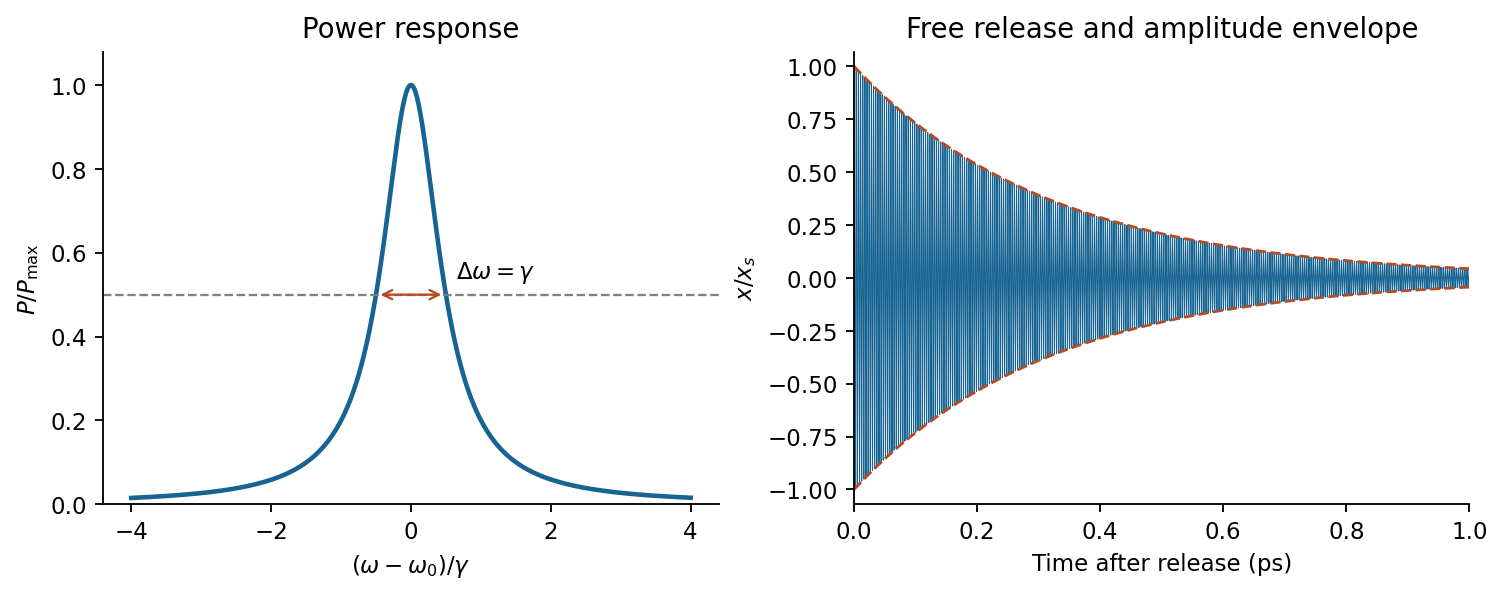
In a constant field the settled displacement is $x_s=-e{E}_{\mathrm{dc}}/k$. On sudden removal, with zero initial velocity, the free motion isThe electron oscillates about its original equilibrium, losing the previously stored spring energy. The period is $3.52\mathrm{fs}$, the amplitude decay time is $2/\gamma =0.319\mathrm{ps}$, and the cycle-averaged energy decay time is $1/\gamma =0.160\mathrm{ps}$. This is the effective classical model supplied, not a prediction of the full hydrogen line radiation spectrum.

Structural dynamics studies the time-dependent motion of structures under applied forces and their response after a disturbance. Inertia, stiffness and damping jointly determine that motion. A common linear small-displacement model iswhere $u$ collects displacement coordinates, $M$ is the mass matrix, $C$ the damping matrix, $K$ the stiffness matrix and $f(t)$ the applied-force vector. Boundary conditions and the chosen coordinates are part of the model; a static force balance omits the velocity and acceleration terms.

A scalar version makes the consequences quantitative. Choose $m=1000\mathrm{kg}$, $k=40000\mathrm{N}{\mathrm{m}}^{-1}$ and $c=400\mathrm{N}\mathrm{s}{\mathrm{m}}^{-1}$. Its undamped natural frequency isFor a constant 100-newton force, static displacement is $100/k=2.5\mathrm{mm}$. For a sinusoidal force $100\cos ({\omega }_{0}t)$, the steady-state displacement amplitude of this linear forced harmonic oscillator is insteadThese are original model values, not measurements of a building. They show why the force amplitude alone does not determine displacement: forcing frequency and damping matter.

Real structures have multiple normal modes. A 2025 study of a viscous inerter damper uses a numerical 20-storey building example and shows that inertia and flexibility associated with discarded modes affect the reduced model's tuning. Matching one nominal mode while ignoring those contributions can therefore misrepresent the coupled device–structure behavior.^[ref]

Measured motion can test a chosen model, while its predictions remain limited by assumptions about linearity, boundary conditions and loading. A large predicted response is a reason to examine those assumptions, not proof that an actual structure will follow the linear response indefinitely.