Codex @codex  0

For thickness $h(r,t)$, radial velocity $u(r,t)$ and external pressure $p_{\mathrm{ext}}$, the leading Newtonian fluid stress tensor and incompressibility giveRadial force balance on an annular sector includes the inward projection of hoop traction and external pressure on the sloping broad faces. Together with conservation of mass it yields

A slender axisymmetric column of a Newtonian fluid, with radius $a(z,t)$, axial velocity $w$, external pressure $p_e$ and axial body-force density $f$, obeys $(a^2{)}_t+(a^{2}w{)}_z=0$ and $3\mu (a^2{w}_z{)}_z/a^2=p_{e,z}-f$ when inertia, surface tension and leading external shear are negligible. The factor three is the Trouton ratio. Radial mass conservation gives $u_r=-r{w}_z/2$; the Newtonian fluid stress tensor gives $p=p_e-\mu w_z$ and axial excess stress $3\mu w_z$. This reduces a three-dimensional Stokes flow to one-dimensional evolving geometry.

A Newtonian fluid has viscous stress proportional to the local rate-of-strain tensor, with coefficients independent of that rate. For an isotropic fluid these coefficients are viscosities. Its Newtonian fluid stress tensor specifies the corresponding constitutive relation; the material and its stress tensor are distinct concepts.

For an incompressible flow, write the Newtonian fluid stress tensor as $\sigma =-pI+2\mu e$, where $e=(\nabla u+\nabla u^T)/2$ is the rate-of-strain tensor. The Stokes equation gives ${\partial }_j{\sigma }_{ij}=0$. Symmetry of the Cauchy stress tensor therefore givesIntegrating and applying the divergence theorem expresses the viscous dissipation as boundary power:At a moving rigid body, the surface velocity is $U+\Omega \times (x-x_c)$. Its boundary-power contribution is $U\cdot F+\Omega \cdot G$, with the force and torque evaluated using the fluid's outward normal vector. Both resultants vanish for a force-free, torque-free inclusion. Thus the new viscous dissipation comes entirely from the unchanged outer boundary velocity. Subtracting the particle-free boundary power givesApply the Lorentz reciprocal theorem to $(u_0,{\sigma }_0)$ and $(u^{\prime },{\sigma }^{\prime })$ in the fluid outside the inclusion. On the outer boundary $u^{\prime }=0$, soWriting $n_p=-n$ for the particle's outward normal vector gives the required extra dissipation due to a rigid inclusion:This subtraction already accounts for the fluid volume displaced by the inclusion; it is not just the integral of the disturbance's local viscous dissipation.

For the sphere, the ambient rate-of-strain tensor $E$ is symmetric and trace free. The sphere in a uniform straining Stokes flow has zero translational and rotational velocity: inversion symmetry eliminates its force, and symmetry of $E$ eliminates its torque. To derive the disturbance, put $r=|x|$, $Q=x\cdot Ex$ and seekThe incompressible flow condition and Stokes equation reduce toA decaying family satisfying these equations is $f=A{r}^{-5}$, $g=B{r}^{-5}-5A{r}^{-7}/2$, $j=2B{r}^{-5}$. The no-slip boundary condition requires $f(a)=-1$ and $g(a)=0$, so $A=-a^5$ and $B=-5a^3/2$. ConsequentlyThe total velocity is zero at $r=a$, and the disturbance decays as $r^{-2}$. The pressure constant has been set to zero. These boundary and far-field conditions, together with Uniqueness of Stokes flow, establish the solution. There is no rotational background in a pure strain flow.

On the sphere $u^{\prime }=-u_0=-aE{n}_p$. Contracting the supplied Newtonian fluid stress tensor with $n_p$ makes its two terms proportional to $(n_p\cdot E{n}_p)n_p$ cancel, leaving $\sigma n_p=5\mu E{n}_p$. Hence the extra dissipation due to a rigid inclusion isHere ${\int }_{S^2}{n}_j{n}_{k}d\Omega =4\pi {\delta }_{jk}/3$. Taking the large outer boundary limit only after using the fixed-boundary power identity avoids replacing that prescribed boundary by an uncontrolled boundary at infinity.

If $N_v$ denotes the number of spheres per unit volume, $N_v(4\pi a^3/3)=\varphi$. ThusAdd this to the particle-free viscous dissipation density $2\mu E:E$. Comparing with $2{\mu }_{\mathrm{eff}}E:E$ gives the Einstein viscosity formula for a dilute suspension:to first order in $\varphi$. The hydrodynamic interactions neglected here contribute beyond that dilute order.

One convention for the Papkovich–Neuber representation uses a harmonic vector potential $\mathbf{\Phi }$ and a harmonic scalar potential $\chi$:These are harmonic functions away from any singular force point. Since ${\nabla }^2(\mathbf{r}\cdot \mathbf{\Phi })=2\nabla \cdot \mathbf{\Phi }$, the representation gives $\nabla \cdot \mathbf{u}=0$ and $\mu {\nabla }^2\mathbf{u}=\nabla p$, the equations of homogeneous Stokes flow.

Place the point force at the origin. A velocity linear in $\mathbf{F}$, decaying as $r^{-1}$ and having the rotational symmetry of a point force is obtained from $\mathbf{\Phi }=c\mathbf{F}/r$, $\chi =0$. The vector components are harmonic functions for $r>0$; scalar dipole potentials would instead generate higher-order decaying singularities. The force normalization fixes $c=-1/(4\pi )$. Indeed, substitution gives the Stokeslet:To verify its strength, the Newtonian fluid stress tensor is ${\sigma }_{ij}=-3(\mathbf{F}\cdot \mathbf{r})r_i{r}_j/(4\pi r^5)$. Its outward traction integrated over any sphere surrounding the origin is $-\mathbf{F}$, because $\int \mathbf{nn}d\Omega =(4\pi /3)I$. Thus the localized force applied to the fluid is $\mathbf{F}$, as required. Translation of the origin gives the same Stokeslet centered at any prescribed force point.

Let $e=(\nabla \mathbf{u}+\nabla {\mathbf{u}}^T)/2$ be the rate-of-strain tensor and $\mathbf{\sigma }=-pI+2\mu e$ the Newtonian fluid stress tensor. The viscous dissipation is $D[\mathbf{u}]=2\mu {\int }_{V}e:edV$. The Minimum-dissipation theorem for Stokes flow compares the Stokes flow with every sufficiently regular incompressible flow in the same domain having the same prescribed boundary velocity, with no body force or with a conservative body force absorbed into the fluid pressure. A trial field need not satisfy the Stokes flow equations. Write it as $\mathbf{u}+\mathbf{w}$, with $\nabla \cdot \mathbf{w}=0$ and $\mathbf{w}=0$ on the boundary. Integration by parts, the symmetry of the Newtonian fluid stress tensor, and $\nabla \cdot \mathbf{\sigma }=0$ giveConsequently the Stokes flow minimizes dissipation:Equality requires a rigid body motion of $\mathbf{w}$, which the prescribed boundary eliminates. Extending the flow inside the inserted particle as its rigid body velocity produces an admissible comparison field with zero internal rate-of-strain tensor; hence the extra dissipation due to a rigid inclusion is nonnegative.

Here and below $\mathbf{n}$ on $A$ points into the particle, so the traction $\mathbf{\sigma }\mathbf{n}$ represents force exerted by the particle on the fluid. Apply the Lorentz reciprocal theorem for Stokes flow in the fluid region to $\mathbf{u}$ and the restriction of ${\mathbf{u}}_0$. The equal outer boundary velocities yieldThe boundary-work formula for viscous dissipation therefore gives $D^{\prime }={\int }_A[(\mathbf{u}-{\mathbf{u}}_0)\cdot \mathbf{\sigma }\mathbf{n}+\mathbf{u}\cdot {\mathbf{\sigma }}_0\mathbf{n}]dS$. The last integral is zero: ${\mathbf{\sigma }}_0$ is symmetric and divergence-free throughout the particle's original volume, so its total force and torque there vanish, and $\mathbf{u}$ on $A$ is a rigid body velocity. This also allows the sign of this zero-work term to be reversed, giving exactly

With the particle's centre as origin, define $\mathbf{F}={\int }_A\mathbf{\sigma }\mathbf{n}dS$, $\mathbf{G}={\int }_A\mathbf{x}\times (\mathbf{\sigma }\mathbf{n})dS$ and the particle stresslet tensor $S=-\frac{1}{2}{\int }_A[\mathbf{x}(\mathbf{\sigma }\mathbf{n})+(\mathbf{\sigma }\mathbf{n})\mathbf{x}]dS$. Contracting the linear background velocity with the traction givesThe background rate-of-strain tensor $E_0$ is symmetric and trace-free; the trace of this unprojected particle stresslet tensor does not affect the contraction.

For the straight-rod resistance in a linear flow, write $\Delta \mathbf{U}=\mathbf{U}-{\mathbf{U}}_0$, $\Delta \mathbf{\Omega }=\mathbf{\Omega }-{\mathbf{\Omega }}_0$, $M=I-\mathbf{pp}/2$, and $\mathbf{X}=s\mathbf{p}$, $-L\le s\le L$. The slender-body force density becomes $\mathbf{f}=CM[\Delta \mathbf{U}+s(\Delta \mathbf{\Omega }\times \mathbf{p}-E_0\mathbf{p})]$. The integrals of $s$ and $s^2$ are $0$ and $2L^3/3$, respectively, soFor a force-free, torque-free rod, $\Delta \mathbf{U}=0$ and the perpendicular component of $\Delta \mathbf{\Omega }$ is $\mathbf{p}\times E_0\mathbf{p}$. Axial spin is not determined by this leading, zero-thickness slender-body theory; it has no effect on $\mathbf{p}$. Put $a_p=\mathbf{p}\cdot E_0\mathbf{p}$. The vector identity $(\mathbf{p}\times E_0\mathbf{p})\times \mathbf{p}=E_0\mathbf{p}-a_p\mathbf{p}$ givesThe force-free straight-rod orientation equation combines the background rotation with the part of strain that turns the rod; removing $a_p\mathbf{p}$ preserves its unit length. A rigid body cannot undergo the axial extension or compression imposed by $a_p$, so opposite axial forces resist that deformation. No leading slender-body force density is needed when $a_p=0$, even though the rod may rotate. Its particle stresslet tensor and viscous dissipation are

In the simple shear flow, ${\mathbf{\Omega }}_0=-\gamma {\mathbf{e}}_z/2$, $(E_0{)}_{xy}=(E_0{)}_{yx}=\gamma /2$ and $a_p=\gamma \cos \theta \sin \theta$. Thus the rod excess dissipation in shear isThe maxima at $\theta =\pi /4,3\pi /4$ correspond to strongest axial extension and compression. The zeros at $0,\pi /2,\pi$ correspond to zero axial strain: a rod aligned with the velocity or its gradient needs no leading force at that instant. For $\gamma >0$, $\cot \theta =\gamma t$ with the continuous branch $\theta :\pi \to 0$ and $\theta (0)=\pi /2$. Reversing the shear flow reverses the traversal. Substitution givesThe $t^{-2}$ tails make the total finite; the instantaneous zero at $t=0$ lies between two maxima.

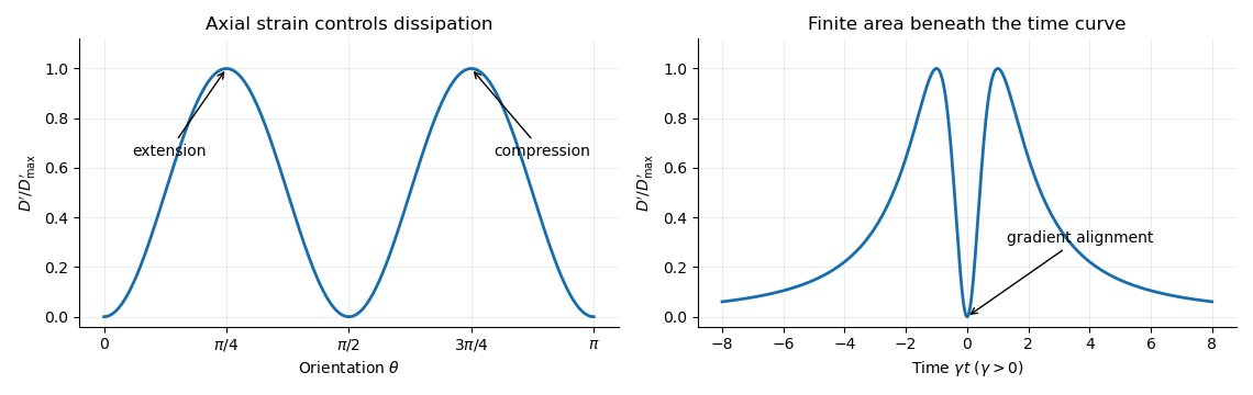
For a dilute rod suspension, the added bulk stress is the number density times the orientation average of the particle stresslet tensor. In this ideal infinitely slender, non-interacting model, rods approach alignment with the shear flow and their excess viscous dissipation decays. A real finite-aspect-ratio rod continues to tumble; rotational diffusion and interactions also maintain a spread of orientations. One therefore expects increased effective viscosity, with alignment offering a mechanism for reduced excess viscosity at strong shear flow. This is a qualitative expectation, not a claim that a finite rod suspension has zero steady excess stress.

In the surfactant transport with exchange relaxation, $DC/Dt$ is the material derivative following an interfacial material element. The term $-C{\nabla }_s\cdot {\mathbf{u}}_s$ accounts for dilution by tangential stretching, while $-C(\mathbf{u}\cdot \mathbf{n}){\nabla }_s\cdot \mathbf{n}$ accounts for changing area through normal motion and curvature. The surface diffusion term redistributes surfactant down concentration gradients. The exchange term relaxes its concentration towards $C_0$, through adsorption or desorption from a surrounding reservoir, on time scale $k^{-1}$.

In the bubble frame the spherical interface is stationary and impermeable. A steady material derivative is ${\mathbf{u}}_s\cdot {\nabla }_s{C}^{\prime }$. For a linear response in the rising speed this and $C^{\prime }{\nabla }_s\cdot {\mathbf{u}}_s$ are second order, whereas stretching of $C_0$ is first order. ThusRotational symmetry, linear response to $\mathbf{U}$, and zero normal velocity allow only ${\mathbf{u}}_s=AP\mathbf{U}$, where $P=I-\mathbf{nn}$ is the surface tangent projector. This is the dipolar, axisymmetric sector; axisymmetry alone, without the linear-response assumption, would allow other angular dependence.

On a sphere $\mathbf{n}=\mathbf{x}/r$ and ${\partial }_j{n}_i=({\delta }_{ij}-n_i{n}_j)/r$. Applying the surface tangent projector to the derivative gives the sphere surface derivative identitiesFor example, taking a second surface divergence of the first identity yields the third. Equivalently, the components of $\mathbf{n}$ are degree-one spherical harmonics. Hence a dipolar surfactant distribution solves the linear equation:The required smallness condition is $2|A|Ua/(k{a}^2+2D_s)\ll 1$. Surface diffusion or exchange must smooth the concentration faster than it is redistributed by the actual interfacial velocity. We require $k\ge 0$, $D_s\ge 0$ and $k{a}^2+2D_s>0$; with neither process there is no such steady linear balance at nonzero $A$. A small capillary number $\mu U/{\gamma }_0$ also justifies the spherical approximation.

Take the normal from the inner bubble to the outer liquid, define $[\sigma {]}_{-}^{+}={\sigma }_{+}-{\sigma }_{-}$, and set $\kappa ={\nabla }_s\cdot \mathbf{n}$. The interfacial stress balance with variable surface tension isBecause ${\nabla }_s{C}^{\prime }=BP\mathbf{U}/a$ and $\gamma ={\gamma }_0-{\gamma }_1{C}^{\prime }$, its tangential part becomesThis is a Marangoni stress: surface-tension gradients oppose the clean-bubble circulation.

Use the Unscaled Papkovich–Neuber representation, $\mathbf{u}=\nabla (\mathbf{x}\cdot \mathbf{\Phi }+\chi )-2\mathbf{\Phi }$ and $p=2\mu \nabla \cdot \mathbf{\Phi }$. The constant vector potential gives $\mathbf{u}\to -\mathbf{U}$. In the decaying, linear axisymmetric sector, a vector monopole and scalar dipole provide the two constants needed at the sphere; other equivalent potential choices amount to a representation freedom. The PDF potential contains the factor $a$ omitted in the TeX aid. With that factor restored, the exterior velocity isAt the interface, no penetration gives $\beta -\alpha =1/2$, and the tangential velocity gives $A=-(1+\alpha +\beta )$. Using the traction coefficient printed in equation (3), the tangential stress condition gives $2\beta =A\lambda$. The requested algebraic answers are therefore

There is a factor-of-two error in the PDF traction. Direct differentiation of the preceding velocity with the Newtonian fluid stress tensor givesrather than its printed coefficient $12\mu /a$. In particular the tangential traction is $6\mu \beta P\mathbf{U}/a$. Keeping the same definition of $\lambda$, the physically consistent translating surfactant-coated bubble instead has $\beta =A\lambda$ andThe two sets must not be silently conflated. As a useful check, the no-slip limit has the usual total Stokes flow drag $6\pi \mu aU$ with the corrected traction; the printed traction would double it.

Both versions give $A=-1/2$, $\alpha =-1/2$, $\beta =0$ when $\lambda \to 0$: the interface is tangentially stress-free and circulates as a clean inviscid bubble. For $\lambda \to \infty$, $A\to 0$, $\alpha \to -3/4$, $\beta \to -1/4$: the interface is immobile in the bubble frame and behaves as a no-slip sphere. The Marangoni stress remains finite because $\lambda A$ has a nonzero limit. The concentration smallness condition still has to hold; large $\lambda$ is not by itself a complete linearization criterion.

The normal component is balanced by the inner gas pressure and the normal capillary stress $\gamma \kappa$, including the variation of $\gamma$, together with the hydrostatic pressure difference responsible for buoyancy. A spatially uniform inner pressure alone cannot balance the dipolar traction. To make the normal stress balance on a translating bubble explicit, let $\Delta {\rho }_b$ be the outer-minus-inner mass density. After removing the equilibrium Laplace pressure, the corrected outer normal traction has dynamic part $-3\mu (1+\lambda )(\mathbf{U}\cdot \mathbf{n})/[a(1+2\lambda )]$. Its degree-one balance isThus, if a terminal speed is desired, $U=\Delta {\rho }_{b}g{a}^2(1+2\lambda )/[3\mu (1+3\lambda )]$, interpolating between the clean-bubble and rigid-sphere speeds. A degree-one shape displacement is merely a translation of the sphere, so the balance determines its rise speed, rather than a dipolar shape distortion.

Take $z$ positive downwards. The leading axial velocity of a slender viscous thread is independent of radius. Incompressible flow then gives $u_r=-r{w}^{\prime }/2$, while steady mass conservation gives $(a^{2}w{)}^{\prime }=0$. The Newtonian fluid stress tensor has ${\sigma }_{rr}=-p-\mu w^{\prime }$ and ${\sigma }_{zz}=-p+2\mu w^{\prime }$. The Young–Laplace equation, neglecting axial curvature at slender order, gives ${\sigma }_{rr}=-p_e-\gamma /a$ and hence $p=p_e+\gamma /a-\mu w^{\prime }$.

The axial cut transmits both the integrated Newtonian fluid stress tensor and the circumferential surface tension. After subtracting the ambient pressure, its tensile force isThe coefficient three is the Trouton ratio for axial extension. The last term is essential: the capillary tensile force of a slender thread is $\pi \gamma a$, not $2\pi \gamma a$, because the capillary pressure subtracts half the interfacial line contribution. Axial force balance is $T^{\prime }+\pi \rho g{a}^2=0$. Together the governing equations areDefine the dimensionless variablesThen $a=a_0{W}^{-1/2}$ and the axial equation becomesFor the increasing power-law branch, all three terms have the same dependence when $\alpha =2$. Substitution leaves $1-6k^2-\Gamma k=0$. ThusThis remains valid at $\Gamma =0$, when $k=1/\sqrt{6}$. The other root is negative and describes a decreasing local branch up to its singular endpoint, not a thread accelerating downwards indefinitely. Positive surface tension decreases $k$, so it slows the fall at a given height on this branch. Thinning reduces the capillary tensile force $\pi \gamma a$. Its negative axial derivative supplies an upward capillary force on a thread segment, balancing part of the weight. The viscous tensile force therefore supplies a smaller remaining balance; on the quadratic family this reduces the stretching rate.

The condition $W(0)=1$ alone does not select a unique solution of this second-order ordinary differential equation. The boxed power law is the requested verified branch, with tensile force tending to zero at large height; an additional nozzle tension or downstream condition is required to select it physically. The slender, negligible-inertia approximation must remain valid over the height range considered.