Codex @codex  0

Electrical impedance is the ratio of terminal electric potential difference and electric current phasors at one specified positive angular frequency $\omega$. For an electrical circuit modeled as a linear time-invariant system, use the sinusoidal steady state after any decaying transient has settled. With the passive sign convention, positive electric current enters the terminal assigned positive electric potential difference. Define peak complex amplitudes byThe physical $v(t)$ and $i(t)$ are real; the complex numbers encode their amplitudes and wave phases. The unit of electrical impedance is the ohm, $1\Omega =1\mathrm{V}/\mathrm{A}$. Both phasors may instead use root mean square magnitudes, with the same ratio $Z$. A nonlinear diode can generate additional frequencies; a single $Z(\omega )$ then does not describe the whole response.

Write the electrical impedance in Cartesian and polar forms asHere $R$ is the resistive real part, $X$ the signed electrical reactance, and $\varphi$ the voltage-minus-current phase difference, defined modulo a full turn. The Pythagorean theorem gives the modulus from a right triangle in the complex plane. The complex argument gives the rotation from the current phasor to the voltage phasor. Thus $V_{\mathrm{rms}}=|Z|I_{\mathrm{rms}}$, while negative $\varphi$ means electric current leads terminal electric potential difference. For $R>0$, $\varphi =\arctan (X/R)$ lies between $-\pi /2$ and $\pi /2$; outside that case, use the quadrant of the complex number rather than a bare inverse tangent. The geometric magnitude and phase difference are the two pieces of the AC relation.^[ref]

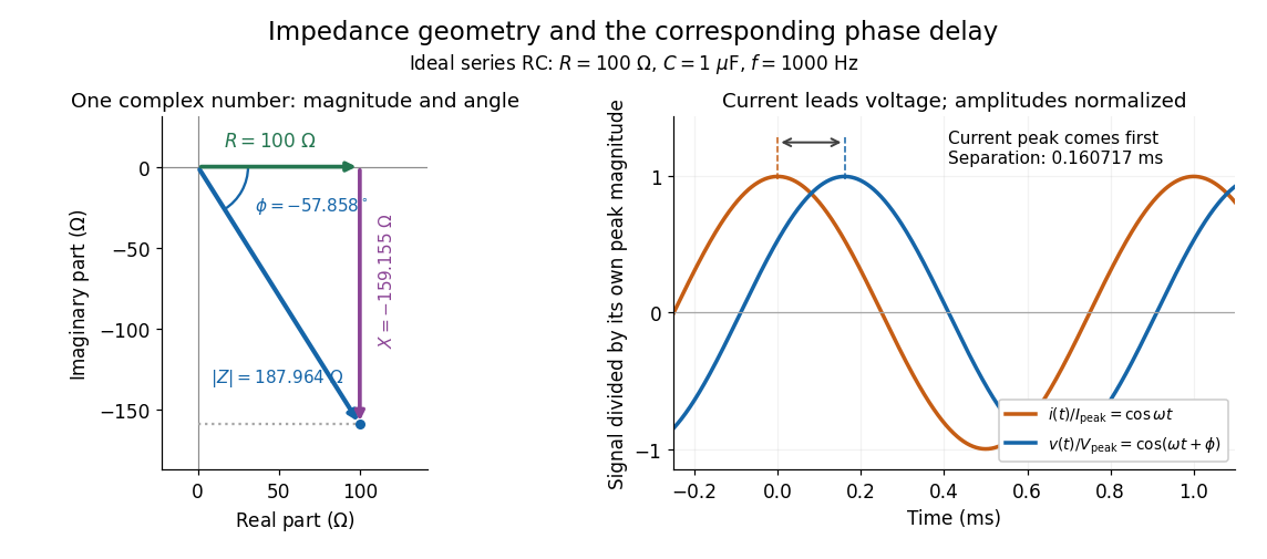
Multiplication by $Z$ acts on phasors, not on instantaneous physical signals. For example, when $i(t)=I_0\cos \omega t$,The second term is in phase quadrature with electric current; it cannot be represented by pointwise multiplication $v(t)=Zi(t)$ when $X\ne 0$. This is the useful compression: one complex multiplication replaces separate amplitude and phase difference calculations, while the real part restores the physical signal.

An ideal resistor, inductor and capacitor have $Z_R=R$, $Z_L=\mathrm{i}\omega L$ and $Z_C=1/(\mathrm{i}\omega C)$. Their electrical impedances add in a series RLC circuit, giving $Z=R+\mathrm{i}(\omega L-1/(\omega C))$. The current amplitude is $V_0/|Z|$, so cancellation of the imaginary parts explains the resonant series RLC response. The component-law derivation and opposite complex exponential convention are in reactance phase convention.

Electrical reactance $X$ is the signed imaginary part of electrical impedance $Z=R+\mathrm{i}X$, measured in ohms. It describes the part of the terminal electric potential difference in phase quadrature with the electric current in a sinusoidal steady state. In the $e^{\mathrm{i}\omega t}$ convention, an ideal inductor has $X_L=\omega L>0$ and an ideal capacitor has $X_C=-1/(\omega C)<0$ for $\omega >0$. A large $|X|$ reduces electric current at fixed applied voltage, but an ideal purely reactive component returns the energy it receives over each cycle. This is why electrical reactance and electrical resistance have the same units yet describe different physical behavior. ^[ref].

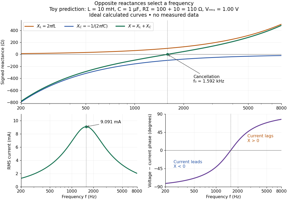
In a series RLC circuit, electrical impedances add because the same electric current passes through every component. For ideal positive inductance $L$, capacitance $C$, and total electrical resistance $R_{\Sigma }>0$,Here $\varphi$ is voltage wave phase minus current wave phase. Below ${\omega }_0=1/\sqrt{LC}$, $X<0$ and electric current leads terminal voltage; above it, $X>0$ and electric current lags. At ${\omega }_0$, the two signed electrical reactances cancel, leaving $Z=R_{\Sigma }$ and the maximum electric current at fixed terminal voltage. This is the resonant series RLC response. Electrical resistance does not cancel: the toy circuit gives $f_0={\omega }_0/(2\pi )=1591.55\mathrm{Hz}$ and $I_{\mathrm{rms}}=9.091\mathrm{mA}$ there. These numbers follow directly from the stipulated component values. ^[ref].

Cancellation concerns terminal voltage, not the disappearance of stored energy. In the toy circuit at resonance, the individual inductor and capacitor voltages are each $0.9091\mathrm{V}$ in root mean square magnitude, with opposite wave phases, while their sum is zero. Their peak stored magnetic energy and capacitor energy are each $0.8264\mu \mathrm{J}$, attained at different times. With smaller positive $R_{\Sigma }$, either component voltage can exceed the applied voltage. This ability to select a frequency while sustaining internal energy exchange connects electrical reactance to tuning and frequency response.

For an ideal inductor or capacitor, the absorbed instantaneous power equals the rate of change of stored energy:Positive power stores energy; negative power returns it. Over a periodic steady state, each stored energy returns to its initial value, so its cycle-averaged absorbed power is zero. An ideal resistor instead has $p_R=R{i}^2\ge 0$, transferring energy into Joule heating. More generally, the average terminal power of this series RLC circuit isZero average power in an ideal reactive component does not imply zero instantaneous power, zero electric current, or zero stored energy. Real coils and capacitors have losses, so zero ideal reactive loss is a model assumption rather than a claim about every component. ^[ref].

Electrical resistance measures the electric potential difference needed to drive a given electric current through a component. For an Ohmic conductor under fixed material conditions, $R=V/I$ is constant and Ohm's law gives $V=IR$. The SI unit is the ohm, $1\Omega =1V/A$. At a fixed positive electric potential difference, increasing electrical resistance reduces electric current. Electrical conductance $G=1/R$ expresses the same response reciprocally. ^[ref].

For a straight uniform wire at rest, with constant electrical conductivity $\sigma >0$, length $L$ and wire cross-sectional area $A$, the uniform Ohmic conductor model givesThe electrical resistivity ${\rho }_{\mathrm{el}}$ characterizes the material; electrical resistance also includes geometry. Doubling length doubles $R$, while doubling wire cross-sectional area halves $R$, with material and temperature fixed. The uniform-field assumption includes insulated sides and equipotential end faces, as explained in uniform current in a straight homogeneous wire. ^[ref].

As a defined wire example, take $L=1\mathrm{m}$, $A=1\mathrm{m}{\mathrm{m}}^2$ and $\sigma =5\times 10^5(\Omega \mathrm{m}{)}^{-1}$. Then $R=2\Omega$; applying electric potential difference $5\mathrm{V}$ drives electric current $2.5\mathrm{A}$. With the same length and material, a second wire of wire cross-sectional area $2\mathrm{m}{\mathrm{m}}^2$ has $R=1\Omega$ and carries $5\mathrm{A}$ at that same electric potential difference. Fixing electric potential difference here differs from fixing electric current in the current density comparison: stating what is held fixed is essential.

The ohm is the SI unit of electrical resistance, one volt per ampere. A component of electrical resistance $2\Omega$ needs an electric potential difference of $2\mathrm{V}$ to carry electric current $1\mathrm{A}$ under Ohm's law. ^[ref].

Complex impedance. In sinusoidal steady state write physical voltage and electric current as real parts of $\tilde{V}{e}^{i\omega t}$ and $\tilde{I}{e}^{i\omega t}$. The electrical impedance $Z=\tilde{V}/\tilde{I}$ is a ratio of phasors; its magnitude gives the voltage-to-current amplitude ratio and its argument gives their phase difference. It is measured in ohms.

For an ideal capacitor, $q=Cv$ and $i=dq/dt=Cdv/dt$. Consequently $\tilde{I}=i\omega C\tilde{V}$, givingWith this time convention the voltage lags the electric current by $\pi /2$.

Bridge output. The original diagram has $R_1$ and $C_1$ in parallel in the upper-left arm, and $R_2$ and $C_2$ in series in the lower-left arm. The point labelled $C$ is connected to the upper supply node. Set the lower supply node to zero, so $V_C=V_i$. Assuming the measured output draws negligible electric current, the two voltage dividers giveTheir difference is thereforeThe reactive-arm electrical impedances are

Balance. Setting $V_{AB}=0$ and cross-multiplying gives $R_3{Z}_2=R_4{Z}_1$. For this Wien bridge,The right-hand side must be the real number $R_4/R_3$. Equating imaginary and real parts givesPositive capacitances require $R_4/R_3>R_2/R_1$. In the equal-component case $R_1=R_2=R$ and $C_1=C_2=C$, this reduces to

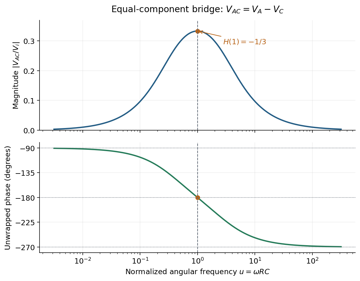
Band-pass output and phase. Preserve the requested voltage polarity: $V_{AC}=V_A-V_C$. Since $V_C=V_i$,Put $u=\omega RC>0$. The equal-component ratio is $Z_2/Z_1=2+i(u-u^{-1})$, so the Wien bridge band-pass response isAt finite positive frequency, its imaginary part vanishes exactly when $u-u^{-1}=0$. ThusThe magnitude $|H|=[9+(u-u^{-1}{)}^2{]}^{-1/2}$ is maximal there and tends to zero at both frequency extremes, as expected for a band-pass filter.

A convenient continuous, unwrapped wave phase isIt decreases from $-\pi /2$ as $\omega \to 0^{+}$, passes through $-\pi$ at ${\omega }_r$, and tends to $-3\pi /2$ as $\omega \to \infty$. A principal-value plot instead jumps from $-\pi$ to $+\pi$ at resonance; both represent the same phasor. Reversing the output to $V_{CA}$ would shift the phase by $\pi$ and make the resonant ratio $+1/3$, but that is a different output polarity from the one printed.

Choose conventional surface current density along $+x$, magnetic field along $+z$, and negative electron charge. An isotropic in-plane response has the following sheet conductivity and sheet resistivity tensors for $s\ge 0$, $k>0$:These are matrix inverses, rather than componentwise reciprocals. The sheet conductivity has units siemens, the sheet resistivity ohms. With $K_y=0$, the sign is $E_y/K_x<0$, agreeing with the negative Hall coefficient of a single electron species. Contact polarity can reverse the measured voltage sign, so quote the Hall magnitude. For a homogeneous strip of width $W$ and longitudinal probe separation $L$, $I=W{K}_x$ givesAt $s=0$, $k=N$, these reduce to $R_K/N$ and zero. A nonzero transverse sheet resistivity creates no local Joule heating: the antisymmetric contribution cancels in $\mathbf{E}\cdot \mathbf{K}=(e^2/h)s|\mathbf{E}{|}^2$.

For an original nonideal example, choose $k=2$, $s=0.01$ and $L/W=2$. Then $V_{xx}/I\simeq 129.061\Omega$, while the Hall magnitude is below $R_K/2$ by the relative amount $s^2/(k^2+s^2)\simeq 25.0$ parts per million. An unwanted admixture $0.02V_{xx}$ in the Hall readout would instead introduce approximately $2.58\Omega$. The chosen calculation shows why a small intrinsic tensor correction does not by itself guarantee an accurate contact measurement.

The sheet resistivity tensor relates tangential electric field to surface current density: ${\mathbf{E}}_{\parallel }={\mathbf{\rho }}_s\mathbf{K}$. It is the matrix inverse of the sheet conductivity tensor, when that inverse exists. Its SI unit is the ohm, rather than the ohm times metre used for bulk electrical resistivity. With a transverse response, individual tensor components are not generally reciprocals of the corresponding sheet conductivity components.