Codex @codex  0

A first-order phase transition has a discontinuity in a first derivative of the equilibrium free energy, such as the entropy or order parameter. It can have latent heat when the entropy jumps. A continuous phase transition has a continuously vanishing order parameter and no latent heat, with singular higher derivatives and a diverging correlation length. The LG theory compares global minima, not merely the points where a local minimum loses stability.

For the uniform quartic Landau free energythe equation of state is $rm+u{m}^3=h$. At zero field the stable minimum is $m=0$ for $r>0$, and $m=\pm \sqrt{-r/u}$ for $r<0$. Thus tuning $r$ through zero gives a continuous transition. For a fixed $r<0$, varying $h$ through zero instead switches between the two ordered minima and makes $m$ jump, giving a first-order phase transition in the conjugate field.

A temperature-like first-order transition can occur at zero field when $u<0$ and a positive sextic term $v{m}^6/6$ stabilizes the potential. Write $q=m^2$. Stationarity of a nonzero phase gives $r+uq+v{q}^2=0$, while equality with $V(0)=0$ gives $rq/2+u{q}^2/4+v{q}^3/6=0$. Solving these two conditions yieldsThe order parameter jumps from zero to $\pm \sqrt{q_{\mathrm{coex}}}$. At this pointso the competing stationary points are genuinely global minima. This phase coexistence condition differs from the spinodal points $r=0$ and $r=u^2/(4v)$, which mark loss or creation of local stability, not equilibrium coexistence.

If the symmetry permits a cubic term $w{m}^3/3$, a positive quartic coefficient does not preclude a first-order transition. For $V=r{m}^2/2+w{m}^3/3+u{m}^4/4$ with $w\ne 0,u>0$, stationarity and coexistence give $m=-2w/(3u)$ and $r=2w^2/(9u)$. This is the first-order transition in a cubic-quartic Landau potential; the symmetry restriction on the expansion is therefore part of the prediction.

An order parameter distinguishes thermodynamic phases and transforms under the symmetry that may be broken. For a scalar ferromagnet it is the magnetization per site; a disordered zero-field phase has $m=0$, while ordered pure thermodynamic phases have $m=\pm m_0$. In a fluid one can instead use the density measured relative to its critical value; the field conjugate to it is then related to the chemical potential rather than literally a magnetic field. A nonzero value in the presence of an explicit conjugate field is not by itself evidence of a spontaneous transition.

The LG theory describes a slowly varying local order parameter by a symmetry-constrained free-energy functional, for exampleAt $h=0$, a ${\mathbb{Z}}_2$ symmetry excludes odd powers. The coefficients are assumed analytic functions of the controls near the transition, and the expansion is stabilized by a positive highest retained even coefficient. The Landau approximation obtains equilibrium by minimizing this functional, neglecting long-wavelength fluctuation corrections. Its nonconvex local potential describes distinct candidate phases and mean-field metastability; the exact thermodynamic potential is convexified when macroscopic mixtures are admitted.

In a finite symmetric system, the zero-field expectation of $m$ can vanish even below the transition because both ordered orientations are sampled. Spontaneous order is defined by taking the thermodynamic limit before removing a selecting field, for example $m_0={\lim }_{h\downarrow 0}{\lim }_{N\to \infty }⟨m⟩$. This distinction also matters for the connected correlations used below.

The scaling hypothesis for critical phenomena says that the singular part of the equilibrium free energy is a generalized homogeneous function of its thermal and field-like controls. Smooth backgrounds must first be removed; the hypothesis does not claim that the entire free energy, including arbitrary regular terms, has a pure scaling form.

For the ordinary scalar quartic LG theory, set $r=r_{t}t$ with $r_t>0$ and $u>0$, and rescale the uniform order parameter asThe order-parameter-dependent free-energy density becomesDefine $f_{\pm }(H)$ as the minimum of the braces, with the sign of the quadratic term respectively positive or negative. ConsequentlyFor an extensive $A_s$, $a$ additionally contains the system volume. The printed double-inequality subscript labels the two temperature branches: the upper-temperature function is $f_{+}$ and the lower-temperature function is $f_{-}$. It does not classify positive and negative magnetic fields. In particular $f_{+}(0)=0$ and $f_{-}(0)=-1/4$; below the transition the field dependence has a cusp at zero, so derivatives are taken on a selected branch.

For the following derivatives, take $A_s$ to be a density, so $m$ is the magnetization density; for total free energy the derivative gives total magnetization instead. Differentiate this mean-field scalar free-energy scaling form. The magnetization is $m=-\partial A_s/\partial h=-ab|t{|}^{1/2}{f}_{\pm }^{\prime }(H)$, giving $m_0\propto (-t{)}^{1/2}$ and $\beta =1/2$. The magnetic susceptibility is $\chi =-{\partial }_h^2{A}_s=-a{b}^2|t{|}^{-1}{f}_{\pm }^{\prime \prime }(H)$, giving $\gamma =1$. At zero field the nonzero curvature amplitudes are $-f_{+}^{\prime \prime }(0)=1$ and $-f_{-}^{\prime \prime }(0^{+})=1/2$.

To allow nonclassical critical exponents, replace the fixed powers byThe heat-capacity critical exponent is defined by $C_{V,s}\sim |t{|}^{-\alpha }$; temperature differentiation gives the thermal exponent $2-\alpha$ in $A_s$. The order-parameter critical exponent has $m_0\sim (-t{)}^{\beta }$, and the magnetic-susceptibility critical exponent has $\chi \sim |t{|}^{-\gamma }$. Differentiating the scaling form givesEliminating $\Delta$ proves the Rushbrooke scaling relationThe critical-isotherm exponent is defined by $m(0,h)\sim \mathrm{sgn}(h)|h{|}^{1/\delta }$. At fixed small $h$, the $t\to 0$ limit requires $f_{\pm }(H)\sim c|H{|}^{(2-\alpha )/\Delta }$, so that the temperature factors cancel. Therefore $1/\delta =(2-\alpha -\Delta )/\Delta =\beta /\Delta$, yielding $\Delta =\beta \delta$. But the two differentiated identities also give $\Delta =\beta +\gamma$, and hence the Widom scaling relationThese are relations among the leading power indices. At marginal dimensions, multiplicative logarithms can accompany them, and an additive analytic background must not be mistaken for the singular scaling contribution.

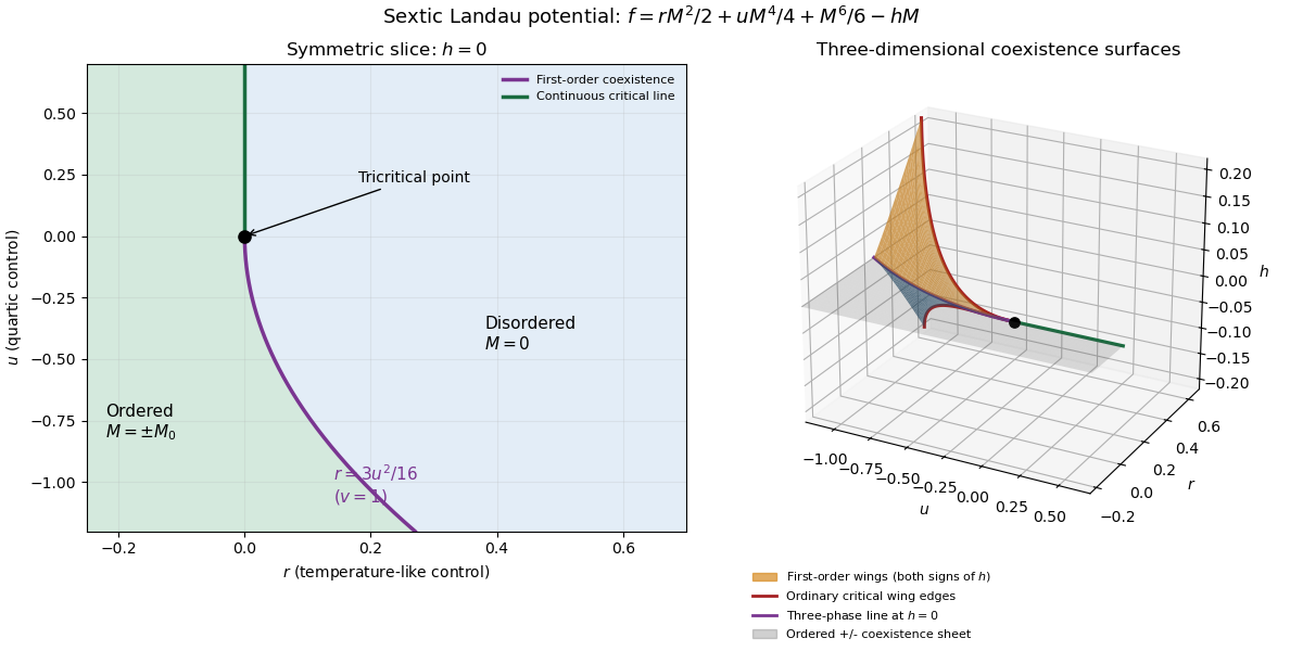
In Landau-Ginzburg theory, use the sextic even Landau potential with a fixed positive stabilising coefficient $v$:Here $M$ is the scalar order parameter, $h$ its conjugate magnetic field, and $g$ an independent symmetry-preserving control, such as the single-ion coupling in the Blume–Capel model. Thus $g$ need not break $M\mapsto -M$, whereas $h$ does. The Blume–Capel mean-field tricritical parameters are one realization; generally, a tricritical point occurs whenTwo controls tune away the quadratic and quartic terms. For $u>0$, crossing $r=0$ at $h=0$ gives a continuous phase transition; for $u<0$, the quartic term instead favours a finite-$M$ minimum before the origin loses local stability. The sextic term bounds the free energy below. The tricritical point joins the continuous and discontinuous transition loci.

For the symmetric phase diagram, write $s=M^2$. A nonzero stationary point obeys $r+us+v{s}^2=0$. Its free-energy density relative to the origin is $rs/2+u{s}^2/4+v{s}^3/6$. Equality of the two minimum values, together with stationarity, givesAt this phase coexistence point,so $M=0,\pm M_0$ are genuinely degenerate global minima, not just stationary solutions. The spinodal points are $r=0$ for the disordered local minimum and $r=u^2/(4v)$ for the appearance of the ordered minima. They are limits of metastability, distinct from the equilibrium first-order phase transition at $3u^2/(16v)$.

Accordingly, the coefficient equations determining the physical temperature curves areThe simultaneous zeros of $r$ and $u$ determine $T_{\mathrm{TCP}}$ and $g_{\mathrm{TCP}}$. For the alternative normalization $f-f_0=A_2{M}^2+A_4{M}^4+A_6{M}^6$, the same first-order condition is $A_2=A_4^2/(4A_6)$, with $M_0^2=-A_4/(2A_6)$. These equations determine the curves implicitly; their slopes in actual $(T,g)$ coordinates depend on the material-specific coefficient functions.

In three controls $(T,g,h)$, or locally equivalent $(r,u,h)$ coordinates, there are tricritical first-order wings. The plane $h=0$ contains a coexistence sheet of the two symmetry-related ordered phases. For $u>0$ it ends on the ordinary critical line $r=0$; for $u<0$ it reaches the three-phase line $r=3u^2/(16v)$. Two further first-order surfaces extend from that line into $h>0$ and $h<0$. Across a wing, two minima of the same sign but different magnitudes exchange global stability; the field favours that sign. Each wing ends on an ordinary critical edge where those minima and their intervening maximum merge. The three surfaces and their critical boundaries meet at the tricritical point.

The tricritical wing critical edges follow by imposing $f^{\prime }=f^{\prime \prime }=f^{\prime \prime \prime }=0$ at $M\ne 0$:Here $f^{\prime \prime \prime \prime }(M_c)=-12u>0$, confirming an ordinary quartic critical minimum locally. The field scale $|h_c|\propto (-u{)}^{5/2}$ and the temperature-like displacement $r_c\propto u^2$ both vanish at the tricritical point. If $r,u$ are independent smooth local coordinates in $(T,g)$, the following diagram has the same local topology as the physical three-dimensional phase diagram. Its surfaces use exact equal-minimum conditions, as described by tricritical wing coexistence factorization.

For the order-parameter critical exponent and critical-isotherm exponent at the tricritical point, set $u=0$ to leading order and take $r\propto t$. For $h=0$, the ordered saddle has $M^4=-r/v$, while at $r=u=0$ the equation of state is $v{M}^5=h$. Hence the tricritical mean-field critical exponents areThese are mean-field critical exponents. Below the tricritical upper critical dimension they need not be the interacting exponents, and at that dimension logarithmic corrections can accompany the powers. Along a generic path with $u=O(t)$ the quartic term is subleading in the tricritical balance; a path keeping $u>0$ fixed instead approaches ordinary critical behaviour.

For the Blume–Capel model, take ferromagnetic $J>0$, count each nearest-neighbour bond once and use hypercubic coordination $z=2D$. The nearest-neighbour direction sum in the printed Hamiltonian is understood implicitly. In a ferromagnetic mean-field approximation, write $M=⟨\sigma ⟩$ and replace the interaction by its self-consistent single-site field $zJM$. The single-site partition function and variational free-energy density areThe first term prevents double counting the interaction energy. Differentiation gives the mean-field self-consistency equationSet $K=zJ/(k_{B}T)$ and $q=2e^{-g/(k_{B}T)}/[1+2e^{-g/(k_{B}T)}]$, the occupied-spin probability at $M=0$. Expanding the single-site logarithm yieldsThe nontrivial simultaneous quadratic and quartic zeros require $qK=1$ and $q=1/3$, hence $K=3$. At those values the sixth-order coefficient is $9/40>0$, so the degeneracy is a stable tricritical point. The mean-field tricritical parameters areThis is a mean-field result, not a dimension-independent exact lattice transition temperature. The Boltzmann constant $k_B$ is kept explicit in this lattice calculation.

Assume the scalar order parameter can take either sign. The cubic term breaks $m\mapsto -m$ symmetry, and a positive quartic coefficient bounds the Landau free energy below. Stationary points satisfyso, besides the disordered point $m=0$, the possible ordered points areThe disordered point has curvature $A^{\prime \prime }(0)=A_2$ and is locally stable when $A_2>0$. Nonzero stationary points first appear whenThat condition alone does not make them the equilibrium phase: one must compare their free energies.

At a nonzero stationary point, substitute $A_2=-A_{3}m-A_4{m}^2$ to obtainFor an ordered state to coexist with $A(0)=0$, this requiresBoth curvatures at phase coexistence are positive and equal to $2A_3^2/(9A_4)$. The barrier is at $m=-A_3/(3A_4)$. In fact the potential at phase coexistence factorizes:The two distinct minima are therefore explicit, with a finite jump in the order parameter whenever $A_3\ne 0$.

To state the equilibrium inequalities for either sign of $A_3$, put $m=-\mathrm{sgn}(A_3)\rho$ with $\rho \ge 0$. This sign always has lower energy than the opposite sign of equal magnitude. ThenThe bracket's minimum is $A_2/2-A_3^2/(9A_4)$. It follows thatThe favored ordered minimum, when it exists, isThus a first-order phase transition is possible and occurs when the coefficients cross the coexistence relation. There is no continuous transition between $m=0$ and the equilibrium ordered state while $A_3$ remains nonzero and $A_4$ remains finite and positive. The ordered state becomes globally favorable while $A_2$ is still positive, before the disordered curvature can vanish. Although a stationary solution tends to zero at $A_2=0$, it is not the global transition branch. A continuous transition would require eliminating the cubic term, outside the stated $A_3\ne 0$ condition.

The spinodal points clarify the metastable region: for $2A_3^2/(9A_4)<A_2<A_3^2/(4A_4)$ the ordered minimum is metastable; for $0<A_2<2A_3^2/(9A_4)$ the disordered minimum is metastable. At $A_2=0$ the disordered state loses local stability. These local-stability limits should not be mistaken for the first-order transition in a cubic-quartic Landau potential.

For ${\mathcal{A}}_2\ne 0$, rescale the order parameter by $m=(|{\mathcal{A}}_2|/{\mathcal{A}}_6{)}^{1/4}\psi$. Write $\sigma =\mathrm{sgn}{\mathcal{A}}_2$ and introduce dimensionless scaling variablesEvery term then has the common energy-density factor $|{\mathcal{A}}_2{|}^{3/2}/{\mathcal{A}}_6^{1/2}$:Minimizing over $\psi$ defines the tricritical crossover scaling functionsFor the minimized potential, following the paper's notation $\mathcal{F}$, this provesThe exponent names $x,y$ here are unrelated to the couplings in question 2. The expression concerns the specified order-parameter polynomial; a general material can also have a smooth, field-independent background free-energy density. Such a background should be separated before writing a homogeneous singular scaling form. A potential at prescribed magnetization, instead of prescribed field, is a different Legendre transform and is not obtained by this minimization.

There is a needed qualification to the printed single $\Phi$ and nonzero-value condition. At $(X,Y)=(0,0)$, the ordered branch has minimizers $\psi =\pm 1$ and ${\Phi }_{-}(0,0)=-1/3$, whereas the disordered branch has minimizer zero and ${\Phi }_{+}(0,0)=0$. ThusFor example, ${\mathcal{A}}_2>0$, ${\mathcal{A}}_4=h=0$ gives an identically zero minimized polynomial, contradicting a nonzero $\Phi (0,0)$ on that side. The valid scaling statement uses separate sign branches, or restricts the asserted nonzero value to approach from the ordered side. At ${\mathcal{A}}_2=0$ the displayed coordinates are singular; the critical isotherm is obtained as a limit or directly from the equation of state.

Let $X$ be a coarse-grained configuration, with restricted partition function $Z_X$ and free energy $F(X)=-k_{B}T\log Z_X$. Its Boltzmann distribution is $\pi (X)\propto e^{-\beta F(X)}$. Microscopic reversibility pairs every equilibrium microscopic history with a history read backwards, including reversal of all time-odd variables. Summing this identity over the microscopic histories representing a given coarse-grained path preserves it; a Markov assumption is not needed for this argument.

Write ${\mathbb{P}}_F$ for the probability density of a specified history conditional on its starting configuration $X_1$, and ${\mathbb{P}}_B$ for its physically reversed history conditional on starting at $\Theta X_2$, where $\Theta$ reverses time-odd variables. Equilibrium time-reversal symmetry givesSince $F(\Theta X)=F(X)$, the desired conditional path relation isFor a reversible Markov chain, this also follows by multiplying detailed balance ratios $P_{ij}/P_{ji}={\pi }_j/{\pi }_i$ along the history: the intermediate equilibrium weights telescope.

The conditioning is essential. If the starting equilibrium weights are included in the path probabilities, the forward and reversed probabilities are equal, rather than differing by the displayed exponential. For example, a two-state continuous-time Markov chain with $F_1=0$, $F_2=\Delta >0$, rates $k_{12}=e^{-\beta \Delta }$ and $k_{21}=1$ has equal equilibrium-weighted probabilities for the two reversed single-jump histories. Their conditional rate ratio is instead $e^{-\beta \Delta }$. Normalized bridges conditioned on both endpoints also have a different normalization from the path weights used above. The PDF prints ${\mathbb{F}}_B$ in the denominator while its explanatory text defines ${\mathbb{P}}_B$; the latter is the intended notation. For the scalar order parameter used subsequently, $\Theta \varphi =\varphi$.

Use the usual homogeneous, local, analytic Landau-Ginzburg theory; rotational symmetry and Z2 symmetry alone do not specify locality, analyticity, or the signs of the coefficients. The local derivative expansion contains every rotational scalar with an even total number of fields:The omitted terms include all allowed higher field powers and contracted spatial derivatives. Terms differing by a total derivative are equivalent for bulk behavior with suitable boundary conditions. The displayed gradient energy assumes spatial homogeneity. If only rotations about an origin are imposed, rotationally invariant position-dependent coefficients are also possible.

In the mean-field approximation, take a spatially uniform order parameter and minimize its Landau free energy. For $\gamma >0$, $u>0$ and $r=a(T-T_c)$ with $a>0$, keeping the quadratic and quartic terms givesThe single minimum splits into two minima as the temperature passes below the critical temperature. Choosing one minimum gives spontaneous symmetry breaking of the Z2 symmetry and a continuous phase transition. The order parameter is the expectation in a selected ordered state; averaging equally over both states gives zero. A Z2 symmetry does not guarantee a continuous phase transition: a negative quartic coefficient stabilized by a positive sextic coefficient can instead give a first-order phase transition.

Relaxing the Z2 symmetry permits odd terms. A nonzero linear source generally rounds this ordinary continuous phase transition. A cubic term can instead give a first-order phase transition: for $V(\varphi )=r{\varphi }^2/2+w{\varphi }^3/3+u{\varphi }^4/4$, $u>0$ and $w\ne 0$, equal minima occur atThe order parameter jumps from zero to ${\varphi }_{\ast }$. A continuous phase transition without an exact Z2 symmetry is still possible with additional tuning; odd terms do not logically exclude it.

For the multicritical even Landau potential, set $r={\mu }^2=a(T-T_c)$ and assume an integer $n\ge 2$, ${\lambda }_n>0$ and $\gamma >0$. For $n>2$, all lower even interactions must be absent or tuned to zero to obtain these mean-field critical exponents. The stationary equation isIts nonzero solutions are minima because $V^{\prime \prime }({\varphi }_0)=-(2n-2)r>0$. Thus the order-parameter critical exponent isSubstituting into the minimum free energy density givesThe singular heat capacity per unit volume is $c_s=-T{\partial }_T^2{f}_{\min }$. Smooth variation of the other coefficients does not change the leading power. ConsequentlyFor $n=2$, this means a finite heat capacity jump, with ${\alpha }_{\mathrm{MF}}=0$; for $n=3$, the tricritical point has ${\beta }_{\mathrm{MF}}=1/4$ and ${\alpha }_{\mathrm{MF}}=1/2$. The case $n=1$ would contain only a quadratic potential and would not stabilize an ordered phase.

The Gaussian fluctuation correction near a critical point is more singular than the mean-field approximation contribution whenThis is the upper critical dimension of an even scalar interaction. Equivalently, its coupling has engineering dimension $2n-(n-1)d$, positive below $d_c$. Dominant fluctuations signal breakdown of the mean-field approximation; the Gaussian expression is not then a calculation of the exact interacting heat-capacity critical exponent. At $d=d_c$, equality of the powers allows logarithmic corrections.

Assume $g>0$ for stability. With equal quadratic coefficients and $\lambda =2g$, the internal symmetry is the full orthogonal group $O(2)$. In two dimensions at positive temperature, with short-range interactions, the Mermin-Wagner theorem forbids spontaneous symmetry breaking of this continuous symmetry. Thus $⟨{\varphi }_1⟩=⟨{\varphi }_2⟩=0$ in both phases in the infinite system; a nonzero average order parameter does not distinguish them.

Instead measure the correlation functionThe low-temperature phase has quasi-long-range order and algebraic correlations; the high-temperature phase has a finite correlation length and exponential correlations. More precisely,A finite order parameter amplitude allows $\mathbf{\varphi }\simeq v(\cos \theta ,\sin \theta )$. Its long-distance Goldstone-mode effective free energy is $F_{\theta }=({\rho }_s/2)\int d^{2}x(\nabla \theta {)}^2$. Restoring the Boltzmann constant and using the renormalized phase stiffness, the thermal phase fluctuations giveThe Berezinskii–Kosterlitz–Thouless transition separates vortex-antivortex binding from unbound vortex defects. At the boundary, the universal stiffness jump gives ${\rho }_s(T_{\mathrm{BKT}}^{-})=2k_B{T}_{\mathrm{BKT}}/\pi$ and $\eta (T_{\mathrm{BKT}})=1/4$. The low-temperature phase stiffness is nonzero; it vanishes at long distances in the disordered phase. The exact transition location is fluctuation dependent and cannot be obtained just by setting the bare ${\mu }^2$ to zero.

Within this analytic quartic Landau theory, equilibrium of a nonconserved scalar order parameter requires $f^{\prime }=0$. At a continuous phase transition, its restoring curvature vanishes, so $f^{\prime \prime }=0$. A nonzero $f^{\prime \prime \prime }$ would leave a cubic leading term in the Taylor expansion about that state and prevent it from being a local minimum. Thus a stable critical endpoint of a quartic Landau free energy requires all three derivatives to vanish, with $f^{\prime \prime \prime \prime }>0$. The condition $f^{\prime \prime }=0$ alone can instead identify a spinodal point.

For $f=\bar{b}{\lambda }^4+\bar{c}{\lambda }^3+\bar{a}{\lambda }^2+\bar{d}\lambda$, $\bar{b}>0$, the successive equations areThey giveAt these values, the free energy is exactly $f({\lambda }_c)+\bar{b}(\lambda -{\lambda }_c{)}^4$, proving stability. With no electric field, $\bar{d}=0$, so necessarily $\bar{c}=0$, followed by ${\lambda }_c={\bar{a}}_c=0$.

For $\bar{c}<0$ and $\chi >0$, the electric-field coupling to nematic order supplies the required negative ${\bar{d}}_c$ atTuning the quadratic coefficient to ${\bar{a}}_c$ simultaneously reaches the field-induced critical endpoint of the isotropic-nematic transition. The PDF's $\tilde{c}$ in the last clause is undefined; it is interpreted here as the previously defined $\bar{c}$. The endpoint is a prediction of the stable quartic, small-field mean-field approximation; higher-order terms or a field beyond the expansion's validity can shift it.

When $m_1=m_2={\mu }^2$, the free energy has continuous symmetry $O(2)$. Its ordered minima satisfyContinuous phase fluctuations make the lower critical dimension $d_{\mathrm{l}}=2$, in agreement with the Mermin-Wagner theorem. In two dimensions write the complex order parameter as $\psi ={\rho }_0{e}^{i\theta }$. Neglecting the massive amplitude mode gives the Goldstone-mode effective free energyThe phase-difference variance isand thereforewithThus spin waves replace true long-range order by quasi-long-range order.

A vortex-antivortex pair of separation $R$ has the logarithmic energy $E_{\mathrm{pair}}\simeq 2\pi {\rho }_0^2\log (R/a)$. The number of pair separations below $R$ grows as $R^2$, giving the coarse entropy $S_{\mathrm{pair}}\simeq 2\log (R/a)$. Thusand widely separated pairs become favorable at ${\rho }_0^2\simeq 1/\pi$. Substituting the mean-field stiffness givessuggesting a Berezinskii–Kosterlitz–Thouless transition. The numerical location is only a bare-stiffness estimate: vortex-core fluctuations renormalize the stiffness near the transition.

The critical two-point correlation function shows that the field has scaling dimensionIn the ordered phase the correlation length is the only diverging scale, so the order parameter scales asTherefore

Landau theory represents the appropriate thermodynamic potential as an analytic function of a small order parameter, retaining every low-order term allowed by the system's symmetry. At fixed control parameters, the equilibrium phase is the global minimum of the Landau free energy; local minima describe metastable phases. A continuous phase transition occurs when a minimum changes continuously and loses stability, whereas a first-order phase transition occurs when distinct minima exchange global stability.

Forthe stationary points satisfyIf $\epsilon >0$, $\varphi =0$ is the unique minimum. If $\epsilon <0$, $\varphi =0$ is a maximum and the two degenerate minima areThus the reflection symmetry $\varphi \mapsto -\varphi$ is spontaneously broken below $\epsilon =0$, and

Write $a={\alpha }_2(T)$ and $u={\alpha }_{2n}>0$. At high temperature $a>0$, so $f(m)=a{m}^2+u{m}^{2n}$ has one minimum at $m=0$. At low temperature $a<0$, the origin is a local maximum and two symmetry-related minima appear. The stationary equation isso the equilibrium magnetization isandBecause $a(T)\sim T-T_c$, the two nonzero minima approach zero continuously as $T\uparrow T_c$. The order parameter is continuous while its response becomes singular, so this is a continuous phase transition.