Codex @codex  0

In a first-order phase transition, two distinct global minima of the Landau free energy have equal values and exchange stability. The equilibrium order parameter jumps, and a first derivative of the equilibrium free energy is discontinuous. Depending on the direction through the phase diagram, that derivative can be magnetization, entropy or another conjugate quantity; a first-order transition need not have latent heat along every chosen path.

In a continuous phase transition, the equilibrium order parameter changes continuously while the curvature at the critical minimum vanishes. For $u>0$ and $h=0$, $M=0$ is stable for $r>0$, but for $r<0$ the stable minima have $M\simeq \pm \sqrt{-r/u}$. The order parameter therefore goes continuously to zero at $r=0$; the inverse magnetic susceptibility vanishes there.

For $u<0$, the sextic term stabilizes the Landau free energy. The nonzero minima can become favorable while $M=0$ still has positive curvature. At $r=3u^2/(16v)>0$ they coexist with $M=0$, so the order parameter jumps to magnitude $\sqrt{-3u/(4v)}$. Finding a stationary point alone does not locate the transition: equilibrium requires comparing the values of all competing minima. Spinodal boundaries describe loss of local stability, not coexistence.

Universality of critical phenomena means that many microscopic models approach the same long-distance renormalization-group fixed point. After repeated coarse-graining, irrelevant operators lose influence, whereas a few relevant operators describe deviations from criticality. Models with the same spatial dimension, order parameter symmetry, interaction range and appropriate relevant controls can therefore have the same universality class despite very different microscopic constituents.

The critical exponents, appropriately normalized scaling functions and certain amplitude ratios are universal. The transition temperature, individual amplitudes, microscopic length scale and analytic background in the free energy are generally nonuniversal. The numerical value assigned to an order parameter also depends on normalization. Landau-Ginzburg theory expresses this distinction by using a common symmetry-allowed functional form while allowing its coefficients to depend on the material. Computing the true critical exponents below the upper critical dimension requires retaining fluctuations, rather than merely minimizing that functional.

The relevant comparison is a short-range, uniaxial Ising ferromagnet and the liquid–gas critical point of water in three dimensions. Both have one real scalar order parameter: magnetization in the ferromagnet and the appropriately shifted density in the fluid. The magnetic field and a suitable pressure/chemical-potential combination provide the corresponding fields conjugate to an order parameter.

The fluid has no exact microscopic spin-reversal symmetry. Nevertheless, at the liquid–gas critical point the first three derivatives of the local thermodynamic potential can be eliminated or tuned by shifting the density and mixing the thermodynamic control variables. The leading stable expansion is then quartic, with the same long-distance renormalization-group fixed point as the three-dimensional short-range Ising model. The microscopic asymmetry produces corrections and analytic mixing of observables, rather than a different leading universality class.

Thus the scalar liquid–gas critical point and the short-range Ising ferromagnet share a universality class. This does not assert that every ferromagnet does: an isotropic vector-spin magnet or one dominated by long-range dipolar interactions can have different critical behavior. Nor does it identify every phase transition of water with its liquid–gas critical point.

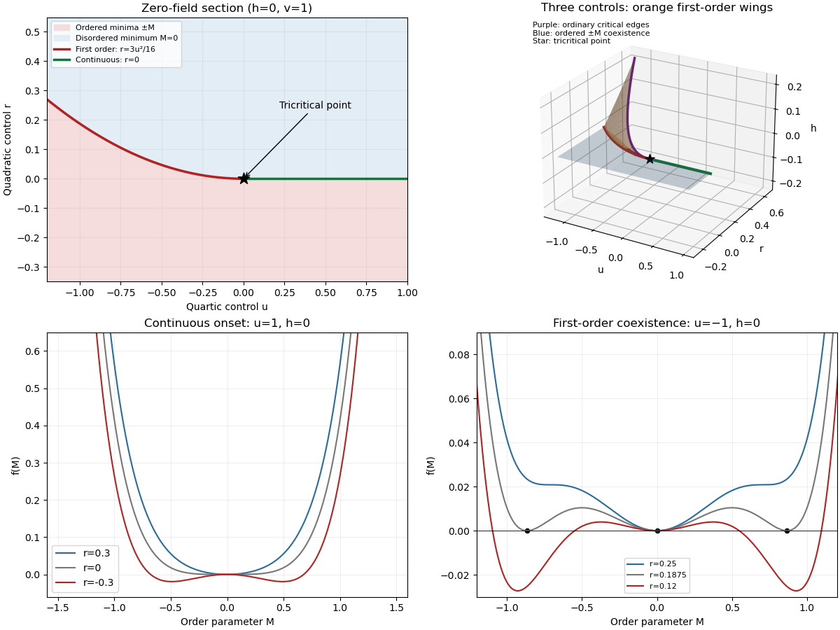
A tricritical point requires two independent even coefficients in the Landau free energy to vanish: $r=u=0$, with $v>0$ providing stability. At $h=0$, the ordinary critical line $r=0,u>0$ meets the tricritical three-phase line $r=3u^2/(16v),u<0$. The order parameter discontinuity along the first-order line is $\sqrt{-3u/(4v)}$, which goes to zero at their meeting.

The positive sextic coefficient makes this a different leading local potential from an ordinary quartic critical point. Consequently its mean-field critical exponents, crossover behavior and upper critical dimension differ. There are two relevant even tuning directions near the tricritical point, in addition to the conjugate odd field. The root solution and labelled phase diagram display the three controls and the tricritical wings; varying $h$ can give a first-order reversal within the ordered coexistence sheet, a first-order weak/strong transition on a wing, or a continuous transition at a wing's ordinary critical edge.

A phase diagram partitions a space of thermodynamic controls into regions with distinct equilibrium phases. Its boundaries indicate phase coexistence or continuous phase transitions; a critical point is a termination of coexistence where the distinction between phases disappears. A concrete three-dimensional control space is $(T,\Delta ,h)$ for the Blume–Capel model: a spin can be $0$ or $\pm 1$, the exchange favors aligned nonzero spins, and $\Delta$ controls the energetic cost of nonzero spins. Varying $\Delta$ changes the balance between a continuous ordering transition and a first-order phase transition. Their meeting is a tricritical point.

Locally, the same structure is displayed by the Landau free energywith three controls $(r,u,h)$. For $u>0$, the line $r=h=0$ consists of ordinary critical points. For $u<0$, equal free energies of $M=0$ and a nonzero stationary point requireEliminating $r$ gives the tricritical three-phase lineHere $M=0$ and both signs of $M$ coexist, with a discontinuous order parameter. Below this line, or below $r=0$ when $u>0$, the plane $h=0$ is an ordered phase coexistence sheet: crossing it reverses the sign of $M$. Two tricritical wings also extend to nonzero $h$, separating weakly and strongly magnetized states of the same sign. Their ordinary critical points satisfy $f^{\prime }=f^{\prime \prime }=f^{\prime \prime \prime }=0$. Since $f^{\prime \prime \prime }=6uM+20v{M}^3$, their tricritical wing critical edges areAt these edges $f^{\prime \prime \prime \prime }=-12u>0$, giving an ordinary quartic critical expansion around $M_c$. All these structures end at the tricritical point $r=u=h=0$. The diagrams show both the zero-field section and the genuinely three-dimensional coexistence structure.

For the final critical exponent calculation, take $r=at$ with $a>0$, $t=(T-T_c)/T_c$, and hold the other controls fixed. At an ordinary critical point, the quartic term dominates the sextic term. For $h=0$ and $r<0$,whereas on the disordered side the singular contribution is zero. Two temperature derivatives give a finite jump in heat capacity, so $\alpha =0$. At $r=0$, the equation of state is $h=u{M}^3+O(M^5)$, so $\delta =3$.

Along the tricritical trajectory $u=0$, the nonzero minimum obeys $M^4=-r/v$ andThus two temperature derivatives produce $|t{|}^{-1/2}$. At $r=u=0$, $h=v{M}^5$. Therefore the mean-field critical exponents areWith $A$ the thermodynamic free energy, the physical sign is $C=-T{\partial }_T^{2}A$, rather than the positive sign printed in the paper. This correction affects the sign of the heat capacity, not its critical exponent. The tricritical result assumes that the independent quartic control is tuned to zero; a generic trajectory through nearby ordinary critical points need not have these exponents.

Let $t,h$ be the thermal and magnetic scaling fields, with eigenvalues $b^{y_t}$ and $b^{y_h}$. After discarding irrelevant variables whose vanishing is nonsingular, the homogeneous singular free-energy density satisfiesChoose $b=|t{|}^{-1/y_t}$. ThenTwo thermal derivatives give the heat-capacity critical exponent; one and two field derivatives give the order-parameter critical exponent and magnetic-susceptibility critical exponent. The correlation-length critical exponent follows directly from the length rescaling. ThusAt $t=0$, choose $b=|h{|}^{-1/y_h}$. Differentiating $f_s(0,h)\propto |h{|}^{D/y_h}$ gives $M\propto \mathrm{sgn}(h)|h{|}^{(D-y_h)/y_h}$, so $\delta =y_h/(D-y_h)$. The order parameter has scaling dimension $x_M=D-y_h$; therefore its critical connected correlation function has power $r^{-2x_M}$. Comparing with $r^{-(D-2+\eta )}$ yieldsThese formulas express the requested critical exponents in terms of the relevant scaling exponents. Their hyperscaling assumptions must be respected: above an upper critical dimension, a dangerously irrelevant coupling can invalidate the free-energy homogeneity used here. Applying the formulas to the Gaussian thinning transformation in the root solution gives the requested Gaussian indices and their physical qualifications.

There is a sign inconsistency in the printed starting energy: its kinetic term uses $\nabla +i{q}_{s}A/\hslash$, while the requested field equation, current and later zero-covariant-derivative condition use $\nabla -i{q}_{s}A/\hslash$. Both conventions can be derived explicitly. Set $D_{\eta }=\nabla -i\eta q_{s}A/\hslash$ for $\eta =\pm 1$; the intended later equations take $\eta =1$, whereas the literal printed energy takes $\eta =-1$.

The magnetic term is $B^2/(2{\mu }_0)$, because $A_{k,j}(A_{k,j}-A_{j,k})=|\nabla \times A{|}^2$. Vary ${\psi }^{\ast }$ independently with compactly supported variations. Integration by parts in the kinetic term givesIn particular $\eta =1$ gives the requested equation. Its conjugate follows from variation in $\psi$.

For variation in $A$, $\delta D_{\eta }\psi =-i\eta q_s\delta A\psi /\hslash$. The kinetic variation is $-j_{\eta }\cdot \delta A$, whereThe magnetic variation is $(\nabla \times B)\cdot \delta A/{\mu }_0$ after integration by parts. ThereforeFor $\eta =1$ this current equals the two displayed forms in the question. For the literal plus-sign energy, $\eta =-1$, the phase-gradient current term has the opposite sign and the field equation contains $D_{-1}^2$. Thus the requested set follows after correcting that one energy sign, not from silently varying inconsistent expressions. This is the gauge-coupling sign in Ginzburg-Landau superconductivity.

Now use the intended convention and write $\psi =\sqrt{n_s}{e}^{i\theta }$ with $n_s>0$. Dividing $D_1\psi =0$ by $\psi$ separates real and imaginary parts:Thus $n_s$ is constant on each connected region. The remaining field equation requires $\alpha +\beta n_s=0$, so for $T<T_c$,The current is $j=(q_s{n}_s/m_s)(\hslash \nabla \theta -q_{s}A)=0$. Taking the curl locally gives $B=0$, hence also solves the Maxwell equation.

For a closed curve on which the order parameter is nonzero and $D_1\psi =0$, Stokes' theorem givesSingle-valuedness of $\psi$ permits phase change $2\pi N$, so the flux quantum magnitude is $h/|q_s|$ (for Cooper pairs, $h/(2|e|)$). There is an important geometric qualification: if the entire spanning surface lies in the smooth zero-field superconducting region assumed above, its flux and the total boundary winding are zero. Nonzero quantized flux occurs through a hole or vortex core where those assumptions do not hold over the spanning surface. More generally, without $j=0$ along the curve, the exact quantized quantity is the fluxoidThus fluxoid and flux quantization in a superconductor are related but are not interchangeable without the current condition.

An order parameter distinguishes phases by a macroscopic quantity that changes at the transition. For an Ising model ferromagnet it is the magnetization per Ising spin, $M=N^{-1}{\sum }_n⟨{\sigma }_n⟩$. At zero magnetic field the statistical Hamiltonian is invariant under spin inversion symmetry. The disordered phase preserves this symmetry, whereas a selected ordered phase has $M\ne 0$ and a spin-reversed partner with $-M$. At finite volume with symmetric boundary conditions the expected value is zero even below the transition; spontaneous magnetization means taking the thermodynamic limit before sending a symmetry-breaking field to zero.

Landau-Ginzburg theory introduces a coarse-grained local order parameter $\varphi (x)$ and a symmetry-constrained free-energy functional. For a short-range system with scalar spin inversion symmetry, a useful expansion isThe coefficients vary smoothly with microscopic control parameters at the level of the Landau approximation; normally $r=A(T-T_c)$ with $A>0$. The gradient term penalizes spatial variation. The magnetic field is conjugate to the order parameter, and odd powers at $h=0$ are excluded by spin inversion symmetry. With $u>0$, the sextic term may be omitted locally; with $u<0$, a stabilizing positive $v$ is essential. The equilibrium uniform order parameter minimizes the local potential $V(M)$, givingThis equation of state follows from minimization, rather than being imposed as an independent assumption. Vector or tensor order parameters and their allowed invariants describe other symmetry classes.

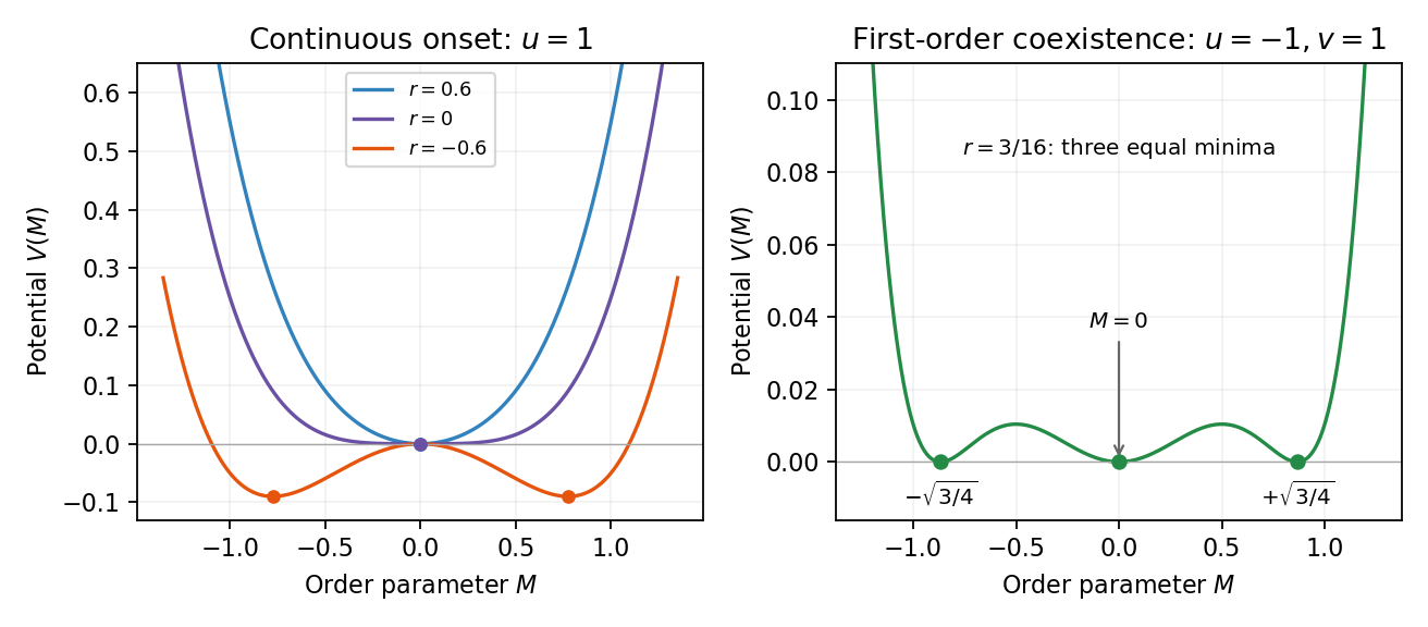
At a continuous phase transition the equilibrium order parameter tends continuously to its critical value, there is no latent heat, and the correlation length diverges. For $u>0$ at zero field, minimizing $V(M)=r{M}^2/2+u{M}^4/4$ gives $M=0$ when $r\ge 0$ and $M=\pm \sqrt{-r/u}$ when $r<0$. These minima join continuously at $r=0$. The minimized singular free-energy density is zero above and $-r^2/(4u)$ below, so its first thermal derivative is continuous, while its second derivative has a finite jump in mean-field approximation.

A first-order phase transition instead has competing minima whose free energies cross while their order parameters remain distinct. The first derivatives of the equilibrium free energy generally jump; along a temperature-driven crossing this gives latent heat. For the symmetric sextic potential with $u<0,v>0$, let $y=M^2>0$. At phase coexistence, the stationary points and equality of the two free energies requireEliminating $r$ gives $-u{y}^2/4-v{y}^3/3=0$, henceAt coexistence $V(M)=v{M}^2(M^2+3u/(4v){)}^2/6$, proving that all three degenerate minima are global. The equilibrium order parameter jumps from zero to one of the two nonzero values even though $r_{\mathrm{coex}}>0$. The disordered minimum loses local stability at $r=0$, and the nonzero stationary points first appear at $r=u^2/(4v)$. These spinodal points delimit metastability and are not the equilibrium transition line. Cubic terms, when symmetry permits them, provide another common route to a first-order transition.

The mean-field approximation replaces each site's fluctuating surroundings by a self-consistent average. On a cubic lattice each spin has coordination number of a lattice $z=2D$, even though summing only over positive basis directions counts each bond once. Write ${\sigma }_n=M+\delta {\sigma }_n$ and drop products of deviations. Each Ising bond becomes ${\sigma }_n{\sigma }_m\simeq M{\sigma }_n+M{\sigma }_m-M^2$, so the approximate statistical Hamiltonian isThe constant corrects counting each bond twice. The resulting independent-spin partition function is $Z_{\mathrm{MF}}=e^{-{\beta }_{T}NzJ{M}^2/2}[2\cosh ({\beta }_{T}zJM){]}^N$, where ${\beta }_T=1/(k_{B}T)$. The one-spin probabilities giveEquating this average with the assumed $M$ givesHere $J>0$ is assumed; a ferromagnetic order parameter is not the appropriate choice for an antiferromagnetic coupling. Put $A=T_c/T$. For $A\le 1$, $\tanh (AM)<AM\le M$ at any $M>0$, so only $M=0$ is possible. For $A>1$, the function $\tanh (AM)-M$ has positive slope at zero, is strictly concave on $M>0$ and is negative at $M=1$. It therefore has exactly one positive zero and a spin-reversed negative zero. Expanding at the bifurcation givesThe transition is continuous, with order-parameter critical exponent $\beta =1/2$. Stability can also be checked from the Bragg-Williams free energy of the Ising model per Ising spin:Its derivative is $-zJM+k_{B}T\mathrm{arctanh}M$, giving the same self-consistency equation. Near zero,The quartic coefficient is positive at $T_c$, the stable minima approach zero continuously, and the minimized free energy has no first-derivative jump. Thus mean-field approximation predicts a second-order transition at $T_c=2DJ/k_B$. This is the mean-field Ising critical bifurcation.

For short-range interactions, large dimension gives many neighbours and suppresses the relative fluctuations of their average. More quantitatively, Gaussian field theory fluctuations averaged over a correlation volume have variance of order ${\xi }^{2-D}$, while the squared ordinary mean-field order parameter is of order $|t|\sim {\xi }^{-2}$. Their ratio is proportional to ${\xi }^{4-D}$. The Ginzburg criterion therefore makes neglect of critical fluctuations asymptotically consistent above four dimensions, inconsistent below four, and marginal at four, where logarithms occur. Large dimension is a route to validity; sufficiently long-range or infinite-range interactions can also produce mean-field behaviour. In low-dimensional short-range systems even the existence and location of a transition can differ from this approximation.

A partition function sums the Boltzmann weights of all states: $Z={\sum }_s{e}^{-{\beta }_{T}H(s)}$ for discrete states, or the corresponding integral for continuous fields. It normalizes equilibrium probabilities. Its physical Helmholtz free energy is $\mathcal{F}=-k_{B}T\log Z$, and its free-energy density is $\mathcal{F}/V$. With a momentum ultraviolet cutoff ${\Lambda }_0$, a scalar-field example isThe normalization of the functional measure and field-independent energy terms must be tracked when discussing absolute free energy.

Choose a smaller cutoff $\Lambda$ and split the field into retained modes ${\varphi }_{<}$ with $|q|<\Lambda$ and eliminated modes ${\varphi }_{>}$ with $\Lambda <|q|<{\Lambda }_0$. Define the Wilsonian coarse-grained statistical Hamiltonian bySubstitution into the partition function proves $Z=\int \mathcal{D}{\varphi }_{<}{e}^{-{\beta }_T{H}_{\Lambda }[{\varphi }_{<}]}$ for every intermediate cutoff. A source retained in this definition similarly preserves long-wavelength connected correlation functions and response. Thus the coefficients in a Hamiltonian density must run with $\Lambda$: the dependence induced by eliminated modes compensates the dependence of the remaining field integral. Holding the original bare coefficients fixed while changing the cutoff would generally change the system. Exact integration generates all interactions allowed by symmetry, including higher powers, derivative terms and an additive constant; a local derivative expansion or a truncation to a few couplings is an extra approximation.

Cutoff independence makes arbitrary intermediate coarse-graining scales unphysical. It allows calculations at the scale of the observable, avoids repeatedly resolving irrelevant short-distance details and exposes the renormalization-group fixed points responsible for universality. A microscopic cutoff, such as a Bravais lattice spacing, can still label a physical microscopic model; taking it to infinity as a continuum limit requires tuning appropriate bare couplings. This is distinct from lowering an intermediate Wilsonian cutoff in a fixed model.

To interpret the zero-cutoff limit, define $M=V^{-1}\int \varphi (x)d^{D}x$, the spatially uniform mode of the order parameter. Keep this mode fixed and integrate the others, rather than integrating over $M$ too. Write $\varphi =M+\eta$, with $\int \eta =0$, and define the constrained order-parameter free energy byIn a finite periodic box, once $\Lambda$ is below the smallest nonzero momentum, all nonconstant modes have been eliminated. The remaining effective energy is $H_{\Lambda }[M]=V{U}_{\Lambda }(M)$, so its defining integral is exactly $Z_M$. Therefore, with consistent normalization,When $\mathcal{H}(\Lambda ,M)$ denotes this uniform effective Hamiltonian density, this is the stated identification of $F(M)$ with its zero-cutoff limit. It requires a free-energy density constrained at fixed $M$, not the unconstrained extensive free energy; all integrated fluctuations and additive constants are included, the zero mode in field theory is retained, and a density for the uniform configuration is well defined. The finite-volume argument avoids an interchange of the thermodynamic and cutoff limits without justification. On a homogeneous pure-phase branch one may use a local potential description, while a thermodynamic limit allowing phase separation can convexify the constrained potential. A bare nonconvex Landau polynomial is accordingly a homogeneous-branch approximation, not a claim that the exact equilibrium Legendre potential stays nonconvex.

In a field $h$, the remaining integral is $Z(h)=\int dM{e}^{-{\beta }_{T}V[F_c(M)-hM]}$, up to the consistently chosen zero-mode measure. The thermodynamic saddle then gives $f(h)={\inf }_M\{F_c(M)-hM\}$ and selects the equilibrium magnetization. Landau theory assumes that the relevant uniform potential can be approximated by a regular analytic expansion in $M$, with symmetry-constrained coefficients, and minimizes it. At tree level the integrated fluctuations are neglected, recovering the familiar bare polynomial. With fluctuations retained, the coefficients run and can become singular near criticality; the zero-cutoff identification of constrained free energy alone does not justify mean-field critical exponents.

For an ordinary short-range scalar thermodynamic critical point, the leading interaction is quartic. Absorb inverse temperature and the gradient coefficient into field normalization and writeScale $x=b{x}^{\prime }$ and $\varphi (x)=b^{-(D-2)/2}{\varphi }^{\prime }(x^{\prime })$ to leave the gradient term invariant. The quartic term changes to $g{b}^{4-D}\int {\varphi }^{\prime 4}/4!$, so its engineering scaling exponent is $4-D$. It is irrelevant at the Gaussian fixed point for $D>4$, relevant for $D<4$, and marginal for $D=4$. HenceThe loop expansion makes the breakdown concrete. A quartic-vertex correction is proportional to $g^2{I}_2(r)$, whereFor $0<D<4$, rescaling $q=\sqrt{r}k$ gives $I_2(r)\sim C_D{r}^{(D-4)/2}$, diverging as $r\to 0$. At $D=4$, radial integration giveswhich is logarithmically divergent. Above four dimensions its infrared limit is finite; the leading cutoff-dependent constant can be absorbed into a coupling renormalization. The effective expansion parameter is thus of order $g{\xi }^{4-D}$ below four, or $g\log (\Lambda \xi )$ at four, since $\xi \sim r^{-1/2}$. It eventually becomes large for any fixed bare interaction in the lower-dimensional critical limit, defeating the uncorrected mean-field expansion. The Ginzburg criterion gives the same threshold by comparing correlation-volume fluctuations with the squared mean order parameter.

Below four dimensions an interacting renormalization-group fixed point can replace the Gaussian fixed point and change critical exponents, provided a continuous transition exists. At four dimensions the interaction is marginal and produces logarithmic corrections: the leading power exponents can remain their mean-field values, so “breakdown” there means that pure mean-field power laws omit those corrections, rather than necessarily that every power exponent changes. Above four the stabilizing quartic interaction is dangerously irrelevant for the ordered phase, explaining why mean-field thermodynamic exponents need not obey naive hyperscaling with the spatial dimension.